NOTES ON BQI 8/2/2024
------------
------------
These notes give a brief description of Burst Quality Indicators
that, as the name implies, are intended to describe the quality
of bursts. Below the BQI are identified in capitals.
These plots, Fig 1, show a
set of figures that illustrate the general burst characteristics.
Fig. 0
 Figs 1 - 3
 Figs 4 - 7
 1) GTK measurements of Bursts
-----------------------------
In general, the characteristics of the burst will be measured
by the number of hits in GTK1. Hits are used rather than tiggers
since they are less influenced by pileup than, for instance,
the trigger rate.
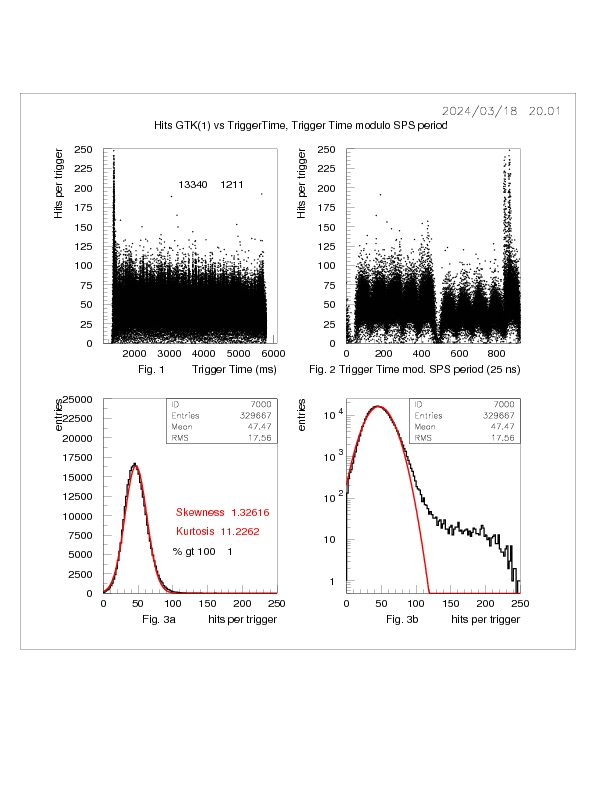
The distribution of the number of hits per trigger in GTK 1 (Fig 3a,b)
is, to a good approximation, Gaussian in shape (Fig 3a),
but a tail is present in many cases as shown by the
log plot (fig 3b).
The Gaussian distribution is described by the MEAN and STANDARD DEVIATION(SD or RMS).
These are ~ 50 hits/trigger and ~15 hits/trigger, respectively.
Notice that the RMS is about a factor 2 larger than expected from the
value of the mean. This is due to the lack uf uniformity of
the spill (see Fig 0, Fig 4) and is further discussed below in relation
to the spill duty factor.
The deviation of the hit distribution from a gaussian distribution
is measured by the SKEWNESS and KURTOSIS parameters.
SKEWNESS = (3rd moment of distribution)/SD**3 0. for Gaussian
KURTOSIS = (4th moment)/SD*4 3. for Gaussian
Skewness measures the asymmetry of the distribution, whereas
kurtosis measures the the tails of the distribution:
leptokurtic = long tails , platykurtic = more peaked than Gaussian.
SKEWNESS and KURTOSIS are highly correlated for these data.
Another parameter that is used is the %HITS GREATER THAN 100.
This gives another measure of the tail of the distribution and is
highly correlated with the skewness and RMS. There is also a weaker correlation
with the RMS and MEAN.
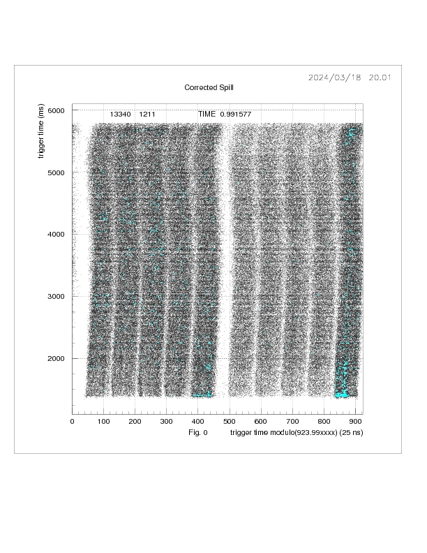
2) The spill distribution.
--------------------------
Fig 0 shows the spill in 2D. The X axis is the trigger time modulo the SPS period
(the folded spill time) with a cubic correction to partially linearize the distribution
in folded spill time. The Y axis is the trigger time.
This plot is also used used to determine the SPS period (see TIME at the top of Fig. 0)..
Evidently the spill is not debunched and there is substantial low frequency noise
modulating the spill.
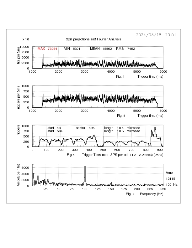
Fig 4 shows the number of hits per trigger in 5ms bins of trigger time.
(An alternative would be number of triggers in 5ms of trigger time
but this shows a reduced variablity due to trigger dead-time, see Fig. 5).
The distribution is characterised by the MEAN , RMS(SD), MAX/MIN
of the spill. The MEAN, RMS and MIN are determined from the 2-5 sec region
of the spill.
The 'noise' in the spill is measured by a Fourier analysis (Fig 7).
This Figure shows that there is a substantial level of low frequency noise,
together with resonances at 50, 100, and 150 Hz.
The BQIs have been chosen to
be the amplitudes of the LOW , 50 and 100 Hz signals since these are the
main contributors to the high RMS of the spill ( and GTK hit distribution).
3)Spill Duty Factor
-------------------
The Spill Duty Factor (SDF) is used to parameterise the uniformity of a particle beam.
This is defined as
(mean intensity)**2/(mean of intensity**2).
Thus a uniform beam would have a SDF of unity and any variations in
in intensty would reduce the SDF.
See Fig 3,page 3, Fig 4, page3
for plots of the SDF for low (12288) and higher (12567) beam intensity
runs, respectively.
Fig. 3 page 3
1) GTK measurements of Bursts
-----------------------------
In general, the characteristics of the burst will be measured
by the number of hits in GTK1. Hits are used rather than tiggers
since they are less influenced by pileup than, for instance,
the trigger rate.
The distribution of the number of hits per trigger in GTK 1 (Fig 3a,b)
is, to a good approximation, Gaussian in shape (Fig 3a),
but a tail is present in many cases as shown by the
log plot (fig 3b).
The Gaussian distribution is described by the MEAN and STANDARD DEVIATION(SD or RMS).
These are ~ 50 hits/trigger and ~15 hits/trigger, respectively.
Notice that the RMS is about a factor 2 larger than expected from the
value of the mean. This is due to the lack uf uniformity of
the spill (see Fig 0, Fig 4) and is further discussed below in relation
to the spill duty factor.
The deviation of the hit distribution from a gaussian distribution
is measured by the SKEWNESS and KURTOSIS parameters.
SKEWNESS = (3rd moment of distribution)/SD**3 0. for Gaussian
KURTOSIS = (4th moment)/SD*4 3. for Gaussian
Skewness measures the asymmetry of the distribution, whereas
kurtosis measures the the tails of the distribution:
leptokurtic = long tails , platykurtic = more peaked than Gaussian.
SKEWNESS and KURTOSIS are highly correlated for these data.
Another parameter that is used is the %HITS GREATER THAN 100.
This gives another measure of the tail of the distribution and is
highly correlated with the skewness and RMS. There is also a weaker correlation
with the RMS and MEAN.
2) The spill distribution.
--------------------------
Fig 0 shows the spill in 2D. The X axis is the trigger time modulo the SPS period
(the folded spill time) with a cubic correction to partially linearize the distribution
in folded spill time. The Y axis is the trigger time.
This plot is also used used to determine the SPS period (see TIME at the top of Fig. 0)..
Evidently the spill is not debunched and there is substantial low frequency noise
modulating the spill.
Fig 4 shows the number of hits per trigger in 5ms bins of trigger time.
(An alternative would be number of triggers in 5ms of trigger time
but this shows a reduced variablity due to trigger dead-time, see Fig. 5).
The distribution is characterised by the MEAN , RMS(SD), MAX/MIN
of the spill. The MEAN, RMS and MIN are determined from the 2-5 sec region
of the spill.
The 'noise' in the spill is measured by a Fourier analysis (Fig 7).
This Figure shows that there is a substantial level of low frequency noise,
together with resonances at 50, 100, and 150 Hz.
The BQIs have been chosen to
be the amplitudes of the LOW , 50 and 100 Hz signals since these are the
main contributors to the high RMS of the spill ( and GTK hit distribution).
3)Spill Duty Factor
-------------------
The Spill Duty Factor (SDF) is used to parameterise the uniformity of a particle beam.
This is defined as
(mean intensity)**2/(mean of intensity**2).
Thus a uniform beam would have a SDF of unity and any variations in
in intensty would reduce the SDF.
See Fig 3,page 3, Fig 4, page3
for plots of the SDF for low (12288) and higher (12567) beam intensity
runs, respectively.
Fig. 3 page 3
 Fig. 4 page 1
 For run 12288 with statistical noise only, the SDF would be expected to
be ~0.98 . A value of ~0.92 is found due to the RMS of the beam being
a factor ~2 larger than the statistical expectation. In addition, some bursts have lower
values of the SDF due to the 100 Hz noise ( see plots on pages 1 and 2 , Fig 3).
Pages 1 and 2 of Fig 3 and Fig 4 show
the correlations between the bunch parameters and their influence, if any, on the SDF.
Fig 3 page 1
For run 12288 with statistical noise only, the SDF would be expected to
be ~0.98 . A value of ~0.92 is found due to the RMS of the beam being
a factor ~2 larger than the statistical expectation. In addition, some bursts have lower
values of the SDF due to the 100 Hz noise ( see plots on pages 1 and 2 , Fig 3).
Pages 1 and 2 of Fig 3 and Fig 4 show
the correlations between the bunch parameters and their influence, if any, on the SDF.
Fig 3 page 1
 Fig 3 page 2
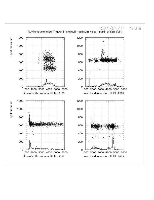
 4)General Run Charactereistics
------------------------------
The lack of uniformity of the spill suggests that a the time of the mamaximum
of the spill, and its value, could be an interesting parameterisation of a run.
Plots of the time of the spill-maximum vs spill maximum are shown in Fig 5
for four runs. The spill maximum/time is determined here from from a plot of trigger time in 5 ms bins.
In the scatterplots each point repesents a bust; the histogram is a projection of the scatterplot on the
time-maximum axis. A uniforn spill would be dispayed as a uniform band of points in the scatterplot.
These four runs illustrate the various departures from uniformity that can occur with intensity peaks
at the start and end of the spill and smooth changes in intensity along the spill.
4)General Run Charactereistics
------------------------------
The lack of uniformity of the spill suggests that a the time of the mamaximum
of the spill, and its value, could be an interesting parameterisation of a run.
Plots of the time of the spill-maximum vs spill maximum are shown in Fig 5
for four runs. The spill maximum/time is determined here from from a plot of trigger time in 5 ms bins.
In the scatterplots each point repesents a bust; the histogram is a projection of the scatterplot on the
time-maximum axis. A uniforn spill would be dispayed as a uniform band of points in the scatterplot.
These four runs illustrate the various departures from uniformity that can occur with intensity peaks
at the start and end of the spill and smooth changes in intensity along the spill.