Analysis of B -> K* µµ
1. The Forward-Backward Asymmetry
On the Bd→K*µ+µ- decay analysis the forward backward asymmetry is defined as the normalised difference between the total number of forward events and the total number of backward events measured. Hence the measurement of the forward backward asymmetry is a simple counting experiment. An event is classified as a forward event if the angle between the muon with positive electric charge and the Bd meson in the dimuon rest frame is smaller than π/2. Otherwise it is considered a backward event. The dependence of the forward backward asymmetry with the dimuon mass squared (Mµµ 2) is also taken into account such that it can be written as in equation 1.
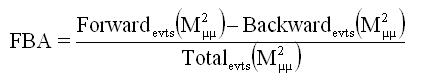
Equation 1: Forward-Backward Asymmetry formula.
where the Forward(Mµµ2 ) is the number of forward events and Backward(Mµ µ2) is the number of backward events both as a function of the dimuon mass squared.
The conventional approach to take into account the dimuon mass dependence when analysing the data is to simply divide the dimuon mass squared range into bins. Here, an unbinned method is proposed which can also be used if the dimuon mass distribution can be described as a smooth curve for both forward and backward events.
2. A Toy Monte Carlo
It is very time consuming to generate events using the full LHCb simulation available. Therefore a Toy Monte Carlo has been used to estimate the LHCb sensitivity to the measurement of the zero point of the forward backward asymmetry. As mentioned before the LHCb simulation includes not just the collisions and decays of the produced particles but also the response of the detectors to the particles passing through its material. In terms of CPU time the more expensive part of the full LHCb Monte Carlo is the detector simulation.
The particle momenta will be measured with very good resolution in the LHCb experiment. The angle between the muon and the Bd meson and invariant mass of the dimuon in the Bd→K* µ+µ- depend only on the particles momenta and therefore their respective resolutions are also expected to be very good.
The detector simulation was then neglected on the Toy Monte Carlo that consisted only in generating signal events within the geometrical acceptance of the detector without simulating the interaction of the particles passing through its material. Using a total of ~7000 events, which is equivalent to one year of data taking, the zero point of the forward backward asymmetry was calculated. The sensitivity to this measurement was calculated by generating a total of 100 sets of events, each one corresponding to one year of data taking and repeating the same procedure.
3. The Unbinned Approach
In general the distribution of a given measurable is estimated by using histograms with fixed bins. These kinds of estimate are discrete, if the number of entries is limited, the estimate is also subject to significant statistical fluctuations. Depending on parameters such as the bin width these estimates of the distribution can be inaccurate or biased. Alternatively a smooth representation of a distribution can also be obtained using statistical estimators. Usually smooth estimators are classified as parametric or non-parametric estimators.
Figure 1 shows an example of the use of a histogram and a non-parametric estimator to represent a given data sample. On the left(or top) plot a histogram with the data entries along the x axis is shown. On the right(or bottom) plot a smooth estimate of the data distribution is shown. It was obtained by assuming a normalised Gaussian distribution for each data entry. The superposition of all Gaussians resulted in the final distribution. This kind of estimator is meant to converge faster with increasing the number of entries than the histogramming technique.
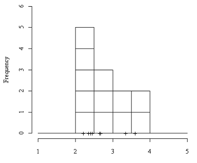
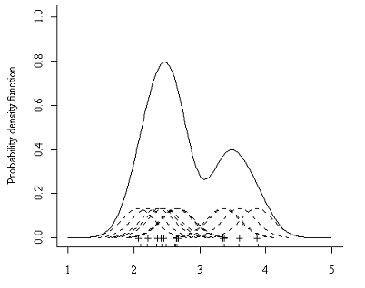
Figure 1: Comparison between histograming and kernel density estimation of a given distribution. The kernel density estimation should represent the distribution better than the histogram.
A typical case of parametric estimator technique is by fitting a known distribution function to a data sample. The quality of the fit can be verified with a χ 2 test. A non-parametric estimator does not assume any knowledge of the data distribution and therefore has the advantage of being model independent. In this analysis a kernel density estimator was used to obtain the distribution of the dimuon mass squared. The estimator used is expressed by equation 2.
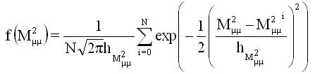
Equation 2: Parzen Estimator with gaussian kernel.
where f(Mµµ2) is the density function estimate, h is the so called smoothness, M iµµ2 is the dimuon mass squared calculated for the i th event and N is the total of events.
Figure 2 shows the dimuon mass squared distribution obtained with both the histogram and kernel density estimation approaches. There is a good agreement between the two methods. Since the kernel density estimator is a smooth function the number of points calculated is not restricted as with the histogram. It provides a better access to the shape of the distribution. The uncertainties on the unbinned method are similar to the binned one. The uncertainties were calculated using 100 sets of events each one being equivalent to one year of data taking.
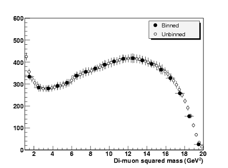
Figure 2: Comparison between histograming and kernel density estimation of the dimuon mass distribution. A better access to the shape of the distribution is obtained with the unbinned method.
The number of forward or backward events can be rewritten using the kernel density estimator as the equation 3.
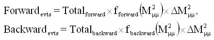
Equation 3: Differential number of forward and backward events as a function of the dimuon mass squared.
Totalforward is the integrated number of forward events and Totalbackward is the integrated number of backward events.
The forward backward asymmetry is then given as a smooth curve on equation 4.
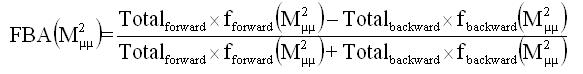
Equation 4: Unbinned formula for the forward backward asymmetry.
Now the forward backward asymmetry can be calculated free of bias or aliasing effects...
4. Data Analysis
In order to use equation 4 the best values to h were calculated using a single set of events equivalent to one year of data taking. The approach employed to evaluate this numbers was a simple χ2. This calculation was implemented in 3 steps.
1- The dimuon mass spectra was calculated for different h values.
A range with suitable values for h was determined and divided in 200 equal steps. The full range of the distribution was calculated using each of these values. The dimuon mass range was also subdivided in very small steps as well.2- The obtained distribution function was compared with a normalized histogram.
The χ2 was defined as in equation 5 to have a smooth comparison between the calculated dimuon mass distribution using the kernel estimator and using a histogram with coarsed bins.
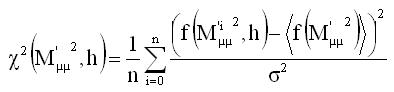
Equation 5: χ2 formula used to estimate the h smoothness.
where ⟨f(M 'µµ 2)⟩ is the density function evaluated by counting the number of events within a range of b~1.6GeV^2 centered at M 'µµ2 . The function f(M i 'µ µ2,h) is the density function calculated for M i 'µµ 2 which is defined as:
Equation 6: Formula used to evaluate the used M i 'µµ2 values in the χ2 calculation.
3- The h values were then optimized as function of dimuon mass values.
By fixing the value of M 'µµ 2 a curve of the χ 2 was drawn as a function of h and the best value for the smoothness determined. Repeating this procedure for the whole range of values of M 'µµ 2 it was possible to determine h as an optimal function of the dimuon mass squared. Figure 3 shows an example of the χ 2 as function of the h values on the top plot and the best values of h as a function of M ' µµ2 on the bottom plot.
Figure 3: The top plot shows the χ2 as a function of the h with fixed M 'µµ2 = 3.0 GeV^2/c^4 . The bottom plot shows h as a function of M 'µµ2 .
Using the obtained curve of h as a function of the dimuon mass the FBA is calculated. In figure 4 the forward backward asymmetry is calculated for 4 different data sets all equivalent to 1 year of data taking. The brick region corresponds to 1σ region and the one green corresponds to 2σ region. The black line is the most probable value for the FBA curve calculated with a single data set and the blue dots correspond to the theoretical value value calculated with about 100 data sets. Observe that the blue dots are most of the time within the 1σ region calculated with a single data set.
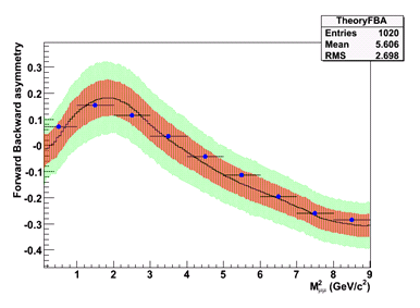
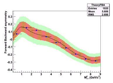

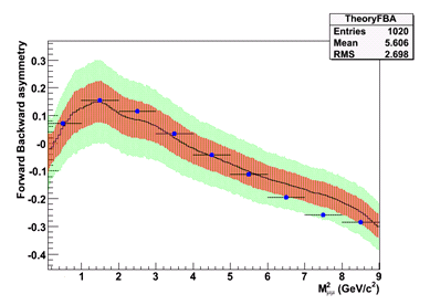
Figure 4: The forward backward asymmetry calculated as a function of M µµ2 for 4 different data sets.
Uncertainties on the FBA are calculated using a simple Monte Carlo based on the equation 6.
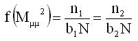
Equation 7: Typical expression used for distribution evaluation.
where n1 and n2 are the number of events within bins of b1 and b 2 both centered at M µµ2. The b 1 and b2 are such that b1 < b2 and b 2 is sufficiently small such that equation 6 is a valid approximation for the dimuon mass density function.
The obtained value for the zero point of the FBA was 4.03+-0.40 GeV^2/c^4.
To be continued...