Velo Alignment Page

Application to the VELO

2. VELO algorithm (Part II)

C. Internal Alignment (STEP 1)

C1. Introduction

As shown by misalignment studies, they are 3 critical degrees of freedom for individual stations: X and Y translations, and Z rotations. Our algorithm should be able to handle precisely at least these 3 parameters. Our sensitivity to the three other DOFs will be slightly lower, but we could tolerate this, at least for the online alignment.

The studies have been done in two steps. First of all, the algorithm is tested with a toy VELO detector model based on the Knossos code . Then, once this step is succesfully fullfilled, we go for a more realistic situation, using minimum bias events within the LHCb classic software chain, along with a VELO misaligned using the LHCb geometry framework.

In this part we present results obtained in the two cases, toy and MC. Our final objective is of course to present here the results obtained with real data (ACDC3 results), this should come at the end of 2006. We will come back to ACDC at the end of this part.

C2. Applying constraints

In the page dedicated to alignment techniques, we saw that Millepede could be used with constraints. Actually this is one of the strongest advantages of global fit methods. However, even in this case, introducing robust constraints is not straightforward, and the choice of equations will not be extensively justified here. We will just briefly explain why we need constraint equations, and how they are introduced in Millepede. More details are available in VELO internal alignment note.

First of all, why do we need to constrain the problem? Because if we don't do so, nothing will prevent linear transformations of the object we want to align. Indeed, during step 1, we align our system using ONLY the track residuals. But these residuals will be the same, wherever the VELO box is. For example, it's easy to understand that the solution is invariant under a VELO box translation.

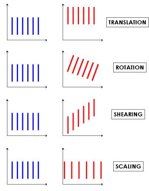
1. Linear global transformations

Translations are the most straightforward example of such transformation, but there are 4 sort of linear global transformations, which are summarized on fig.1. In 3 dimensions, we thus have 12 possible global deformations. However, due to VELO station structure, we could neglect three of them at the first order: shearing in the XY plane, and scaling of the X and Y axis.

Hence we will have to constrain 9 possible deformations: 3 rotations, 3 translations, 2 shearings and scaling of the Z axis. In fact, as it will be difficult, in the VELO context, to disentangle X and Y rotations from YZ and XZ shearing, this number might be reduced to 7 equations.

Now that we now that the constraints are useful, we need to know how they are defined. In the next part, we consider the translation example, easier to handle. For a more complete description, see this HERA-b note.

In each part we will determine a certain number of misalignment constants, 3xN_module translations and 3xN_module rotations.

If all the modules in one half are in their nominal position, one have dx = 0 for each of them, and then, <dx> = 0. It's of course not the case before the alignment, and we even might have a global offset: <dx> = Dx.

Then, if one want to avoid global translation along X axis during the alignment procedure, one should fix the following constraint equation:

<dx> = Dx

The only problem is that we don't know Dx prior to the alignment, that's what we will be looking for during STEP2 !!! In order to solve this problem we use the canonical formalism. The idea behind this is to measure a parameter dx' instead of dx, with dx' defined as:

dx' = dx - Dx

By definition we get:

<dx'> = 0

Here we could define our equation without any problem... In a more general fashion, idea behind the canonical formalism is that we are looking for 'offset-free' misalignments when aligning by tracks, and that those misalignments, by definition, are easily constrained.

C3. Linearizing the system

In order to fulfill Millepede requirements, one needs:

1. Tracks with at least 3 (R,Phi) doublets.
2. For each doublet, X, Y, Z, and error(X,Y), computed as follows:
X = R cos(Phi)

Y = R sin(Phi)

Z = Z(Rsensor)

err_X = sqrt((X*err_R)^2+(Y*err_Phi)^2)/R

err_Y = sqrt((Y*err_R)^2+(X*err_Phi)^2)/R

The choice of Z is justified by the fact that we could consider that Phi(Rsensor)=Phi(Phisensor) at the first order. However this relation, which is clearly not valable for R, could also false for Phi in case of tracks not coming exactly from the beam, like beam halo tracks. To this end a correction, based on track parameters (states), is applied to the Phi value before the spacepoint creation.

C4. STEP1 with TOY model

...Not yet updated...

C5. STEP1 on MC events: effect on misalignments

Following plots were obtained using the GAUDI implementation of the alignment code. 200 sets of 5000 minimum bias events have been produced, each with one different set of misalignments. Misalignments are chosen randomly within a gaussian, the gaussian width setting the scale of the misalignment. For the runs presented here, the scales have been defined as follows:

___________________

1. Module translations (X,Y,Z) : 30 micrometers
2. Module rotations (X,Y,Z) : 2 milliradians

3. Box translations (X,Y) : 100 micrometers
4. Box translations (Z) : 50 micrometers
5. Box rotations (X,Y) : 0.5 milliradian
6. Box rotations (Z) : 1 milliradian
___________________

The 200 sets of events are generated, digitized, and reconstructed within LHCb v20r4 environment, using Gauss v24r7, Boole v11r5, and Brunel v30r2.

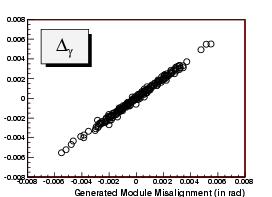
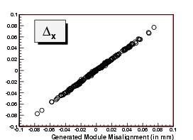
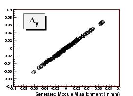
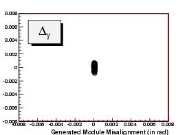
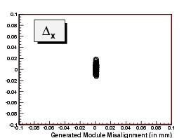
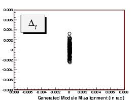
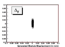
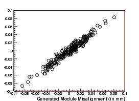
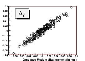
On figs. 2 and 3 are compared the generated and reconstructed misalignment parameters, for right and left halves respectively. All the modules are aligned, ie 21 elements, are taken into account here. Results for all 6 degrees of freedom are shown here (Translations on the left, rotations on the right). As expected, the 3 most sensitive degrees of freedom are well estimated, as the others are not so precisely reconstructed. One retrieve more or less the same type of results than those obtained with the toy, which is quite encouraging.

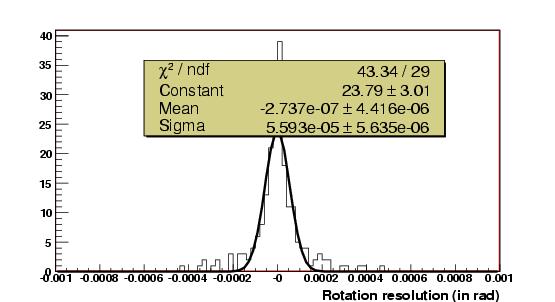
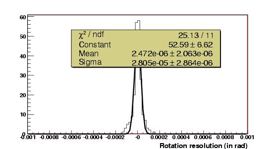
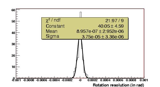
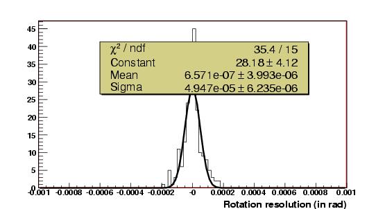
2. Step 1 effect on misalignments (right half).

3. Step 1 effect on misalignments (left half).

Resolution fits, for relevant DOFs, are shown on fig.4.

4. Step 1 resolution for the major DOFs.

These fits lead us to few preliminary remarks. First of all, we observe a good stability for dx and dy translations. These two DOFs have been put together on figures 2 and 4, and it's clear that they are well retrieved. The gaussian fit of fig. 4 confirms this, with a width of about 4 micrometers. The situation is also very satisfying for z rotation, and a 0.3 milliradian precision is obtained, which is well within the trigger requirements, and even pretty correct for reconstruction purposes.

The good news here is that those results could only been improved by the adjunction of halo tracks, in particular in the backward area.

C6. STEP1 on MC events: effect on residuals

After STEP1, as only the station misalignments are affecting the track fit, one should be able to measure the FINAL track residuals. The STEP2 shouldn't change them, as it only affects the primary vertex resolution.

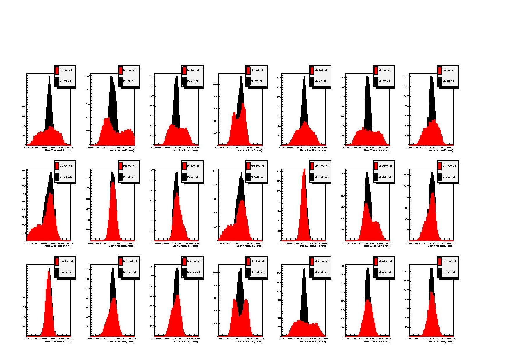
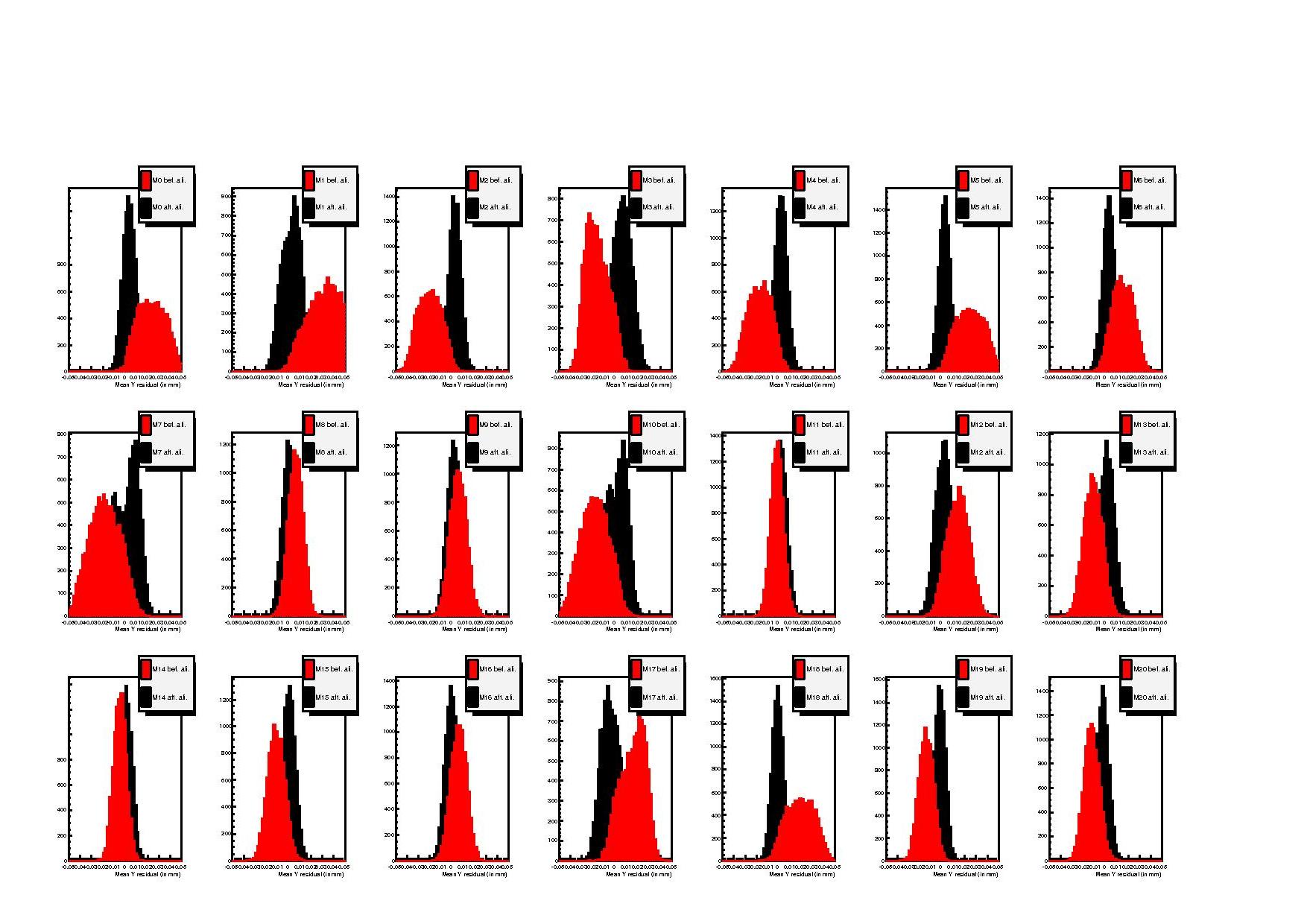
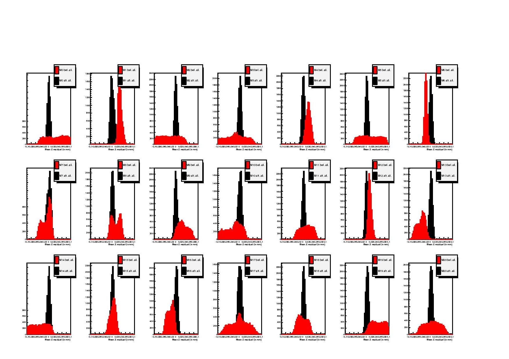
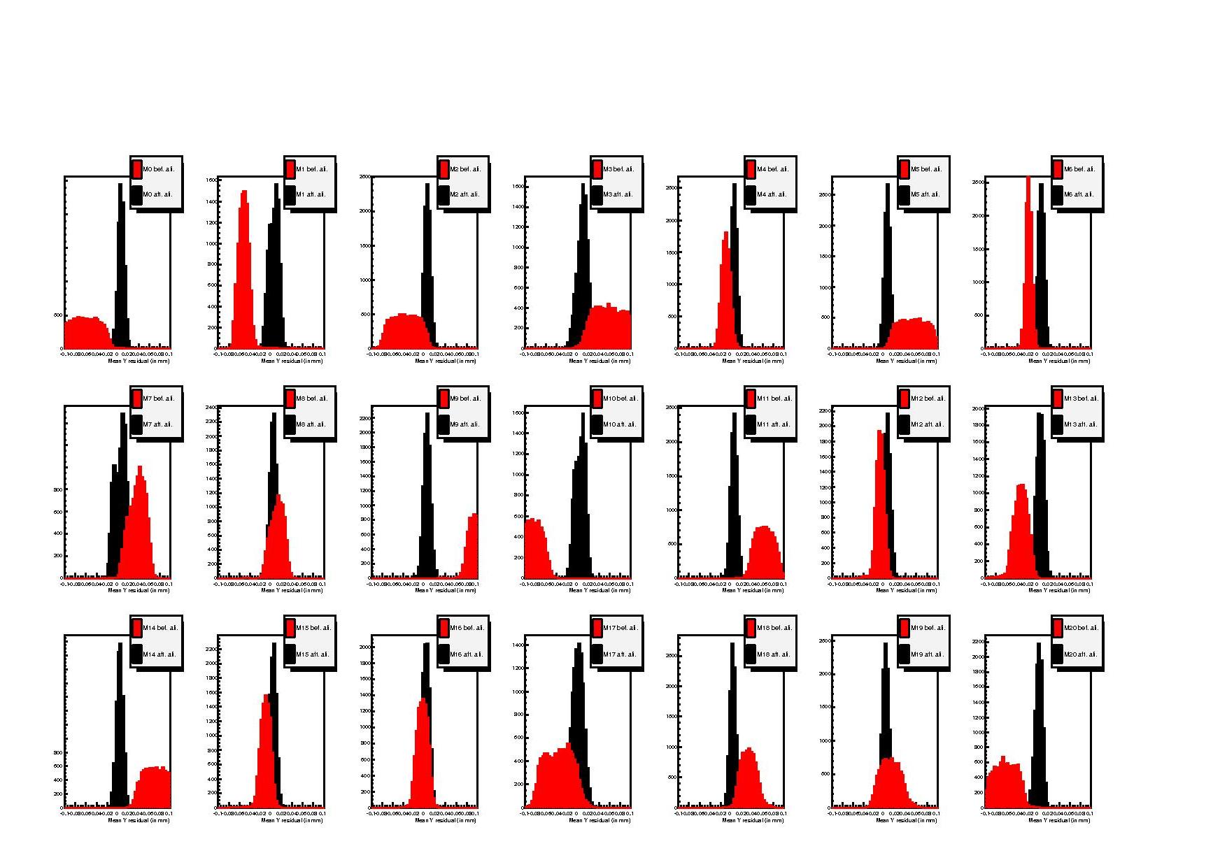
Residuals are monitored via a track control sample stored during the alignment process. A set of 1000 tracks is extracted from the trackstore, these tracks are of course not used for the alignment. Track residuals are then measured before and after the internal alignment process, and results are stored in an ntuple. Then, a small root macro produces the plots below, which could be used to control the alignment. Figures 5 to 8 show the different situations, ie X and Y residuals for both halves, respectively before (top) and after (bottom) the alignment, for one set of misalignments. Thus we clearly see the positive effect of alignment for EACH module.

5. Left X residuals.

6. Left Y residuals.

7. Right X residuals.

8. Right Y residuals.

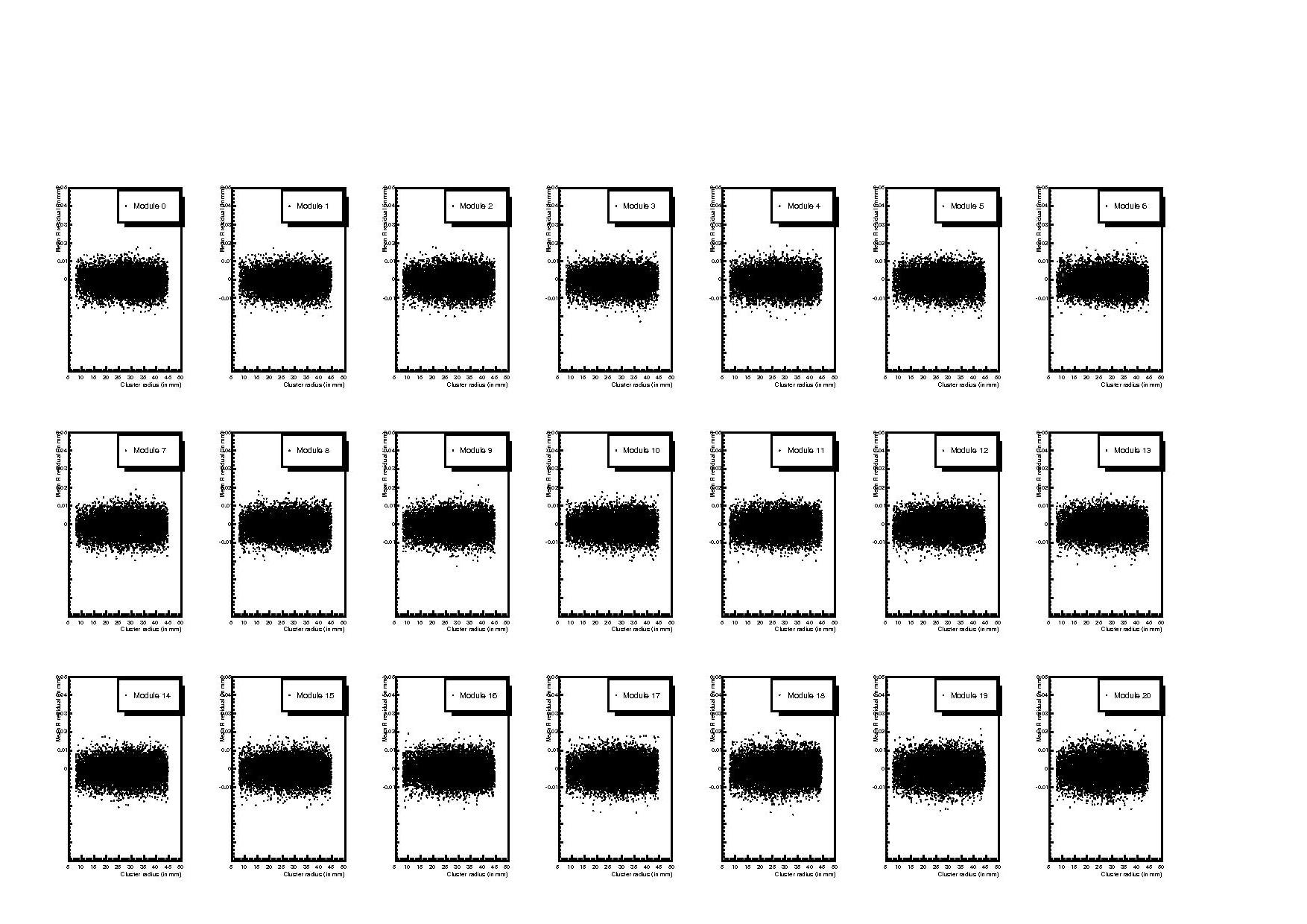
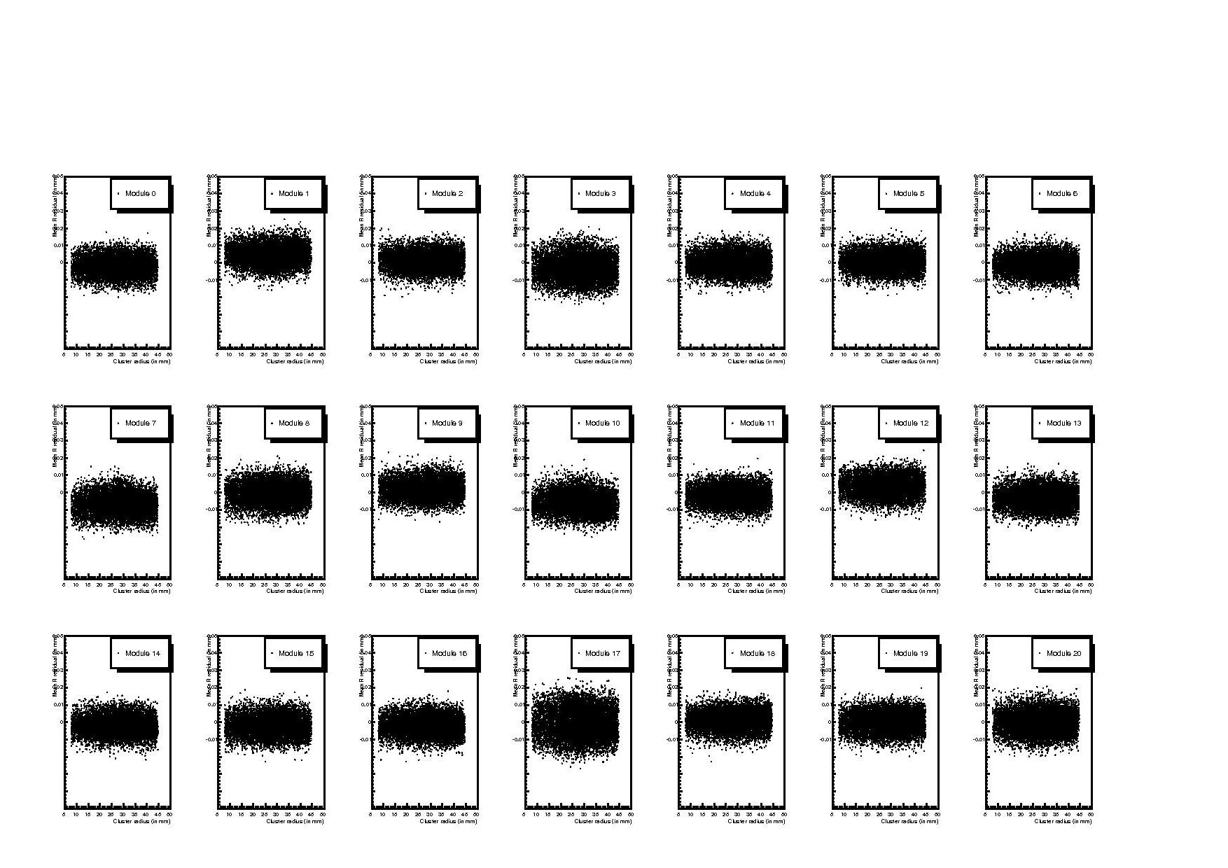
These plots demonstrate the effect of internal alignment for one run, but what about all the runs? This is what is shown on fig.9, where the mean residual values for each modules, for all 200 runs, both before and after STEP1, is shown below.

9. STEP1 effect on residuals

What comes out from fig.9 is that STEP1 has the expected effect on residuals. Mean values are all moved to zero, resolution going from ~20 micrometers to ~3 micrometer. That's exactly what we are waiting from our alignment, so that's quite good. System test using real data are the next step.

C7. System tests preparation. ACDC3 alignment

ACDC3 is expected to happen during Autumn 2006. It consists into a beam test involving a complete VELO half, ie 21 modules. This will be the very first occasion to test the STEP1 alignment with real data. Eventually this is intended to test the full VELO software chain, from data-taking to alignment.

As the tracks used in this test will not have the same topology than the classic one, a specific pattern recognition algorithm hs been developed to reconstruct them: PatVeloGeneric. This code could be also considered as a first version of the Halo track pattern recognition, and is now part of the PatVelo package.

As in the previous case, 200 sets of 10000 misaligned ParticleGun events (within ACDC3 geometry) have been produced. Misalignment scales are the same than in the previous part. Pions are shooted in (X,Y) = (0,0) position, then they interact with iron cylindrical target placed along the beamline. Resulting particles are recovered into VELO half. Track are then reconstructed via PatVeloGeneric, and STEP1 alignment is performed.

Alignment results are shown on fig. 10 (generated vs. reconstructed) and 11 (resolutions). They are comparable to results obtained with MC events. Small differences still need to be understood, but preliminary results are good.

10. Step 1 effect on misalignments.

11. Step 1 resolution for the major DOFs.

As expected, the result get slightly better if the particle are shooted directly into the modules (classic testbeam setup). Fig. 12 and 13.

12. Step 1 effect on misalignments (classic TBeam setup).

13. Step 1 resolution for the major DOFs (classic TBeam setup).

C8. Sensor misalignments: a primary look with the toy

A 'VELO-like' version of the standalone code has been constantly developped in parallel with the MC studies. This version now includes:

1. A realistic geometry : two sets of 42 R/Phi sensors are defined, with a reasonably correct shape. Sensor thickness and resolution could be defined by the user.
2. Realistic tracking information : as in real life, track is reconstructed based on the R and Phi information collected on R and Phi sensors. Cluster error is defined as (StripPitch)/sqrt(12). However strips are NOT defined (--> small cluster position bias).
3. Track residuals before and after alignment are computed and stored in an nTuple. This nTuple has the SAME format than the one produced by the classic alignment software, so that the SAME macros can be used.
4. Everything could be misaligned, ie modules but also sensors. We could also choose if we know the R/Phi misalignments beforehand (via survey), or not.

Using this it is possible to make very quick tests on sensor alignment. These tests will be compared with current MC studies, but they could already give some interesting hints on we could handle R/Phi misalignments.

The tests were made on 2 very simple configurations:

1. Sensor misalignments only, no modules misalignments : scale of the R/Phi misalignments are dX=dY=10microns, dZ=100microns, dA=dB=2mrad and dC=1mrad.
2. Same as 1., but adding modules misalignments : scale of the modules misalignments are dX=dY=dZ=30microns, dA=dB=dC=2mrad.

In each case, 2 runs of 10000 straights tracks are generated: first run is without survey information (don't know Si/Si misalignment), second run is with survey information. The plots presented below show the different results on spacepoints and clusters residuals. Results are presented only for one box.

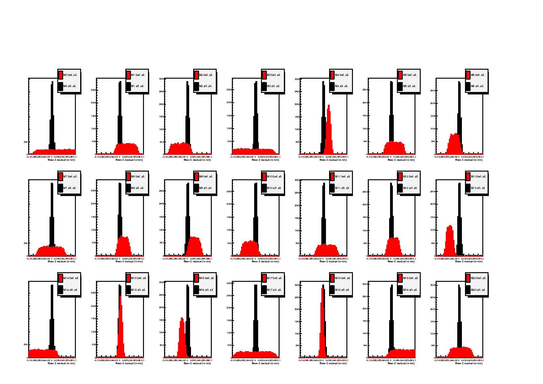
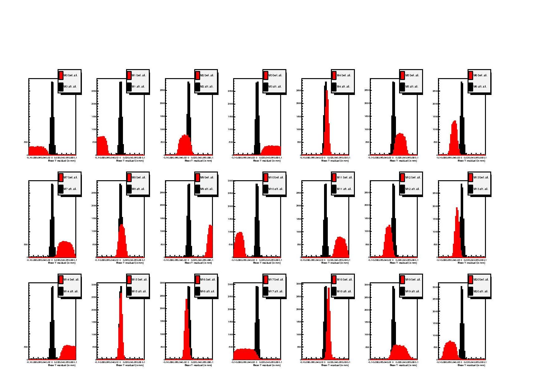
14a to f. Results before and after alignment. Sensors misalignments only, no survey information.

15a to f. Results before and after alignment. Sensors misalignments only, survey information included.

16a to f. Results before and after alignment. Sensors+Modules misalignments, no survey information.

17a to f. Results before and after alignment. Sensors+Modules misalignments, survey information included.

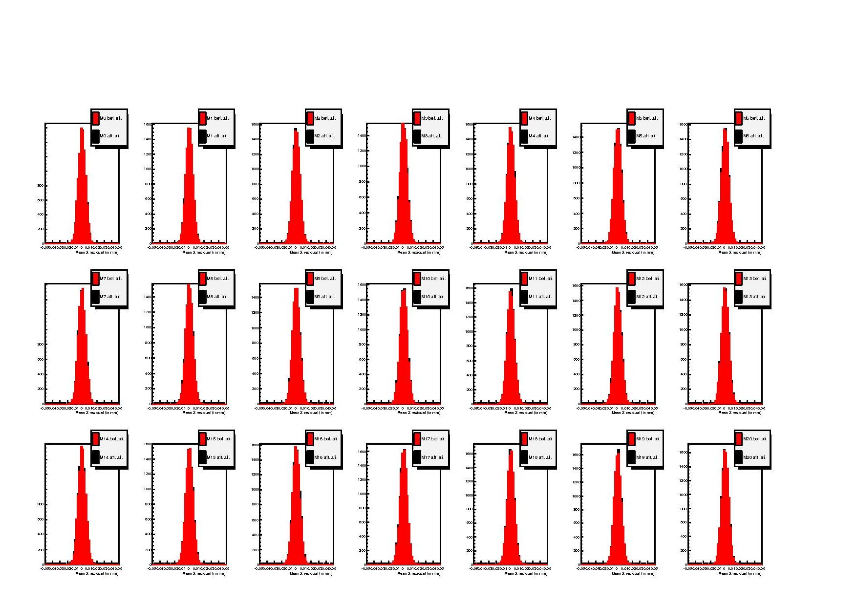
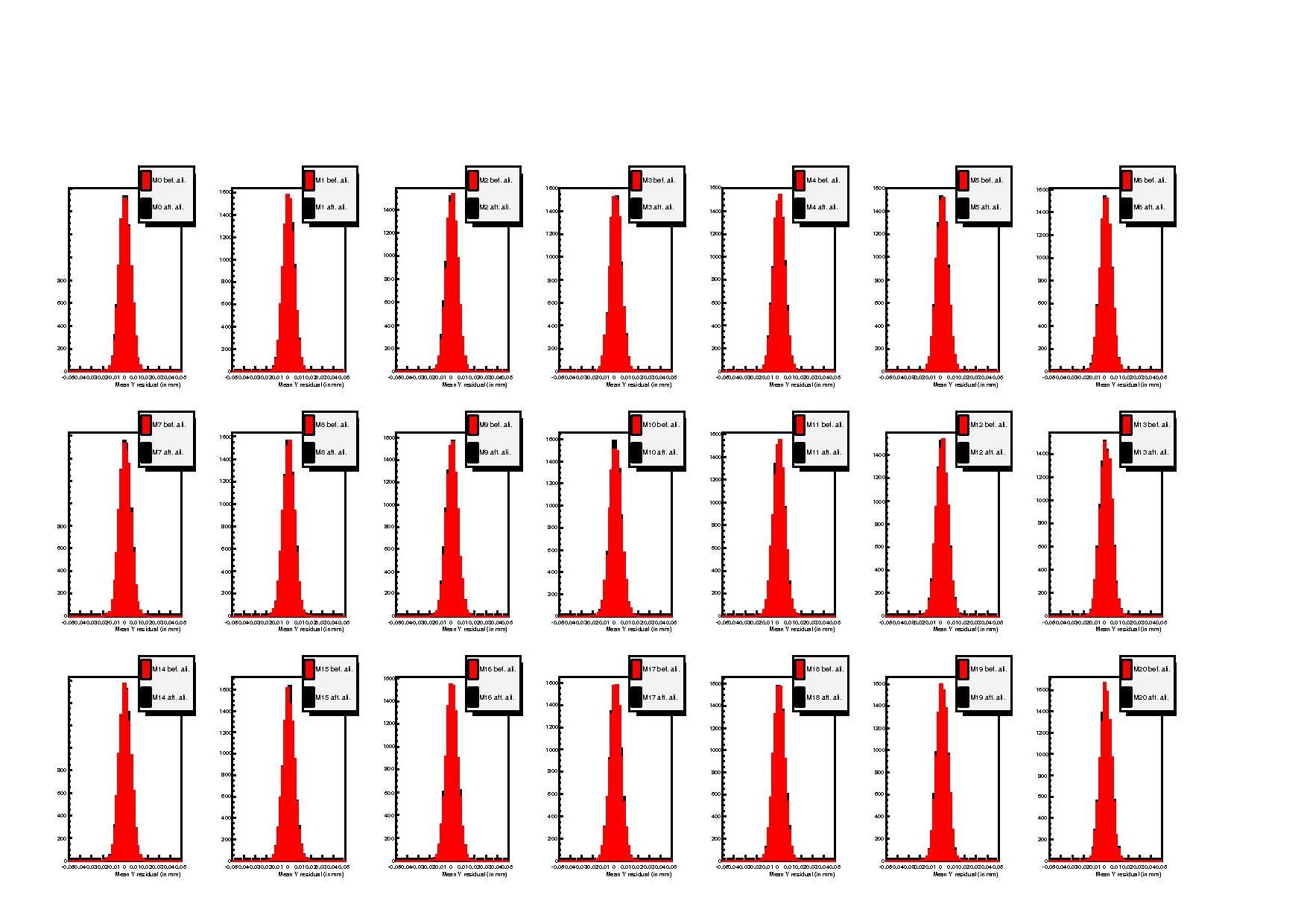
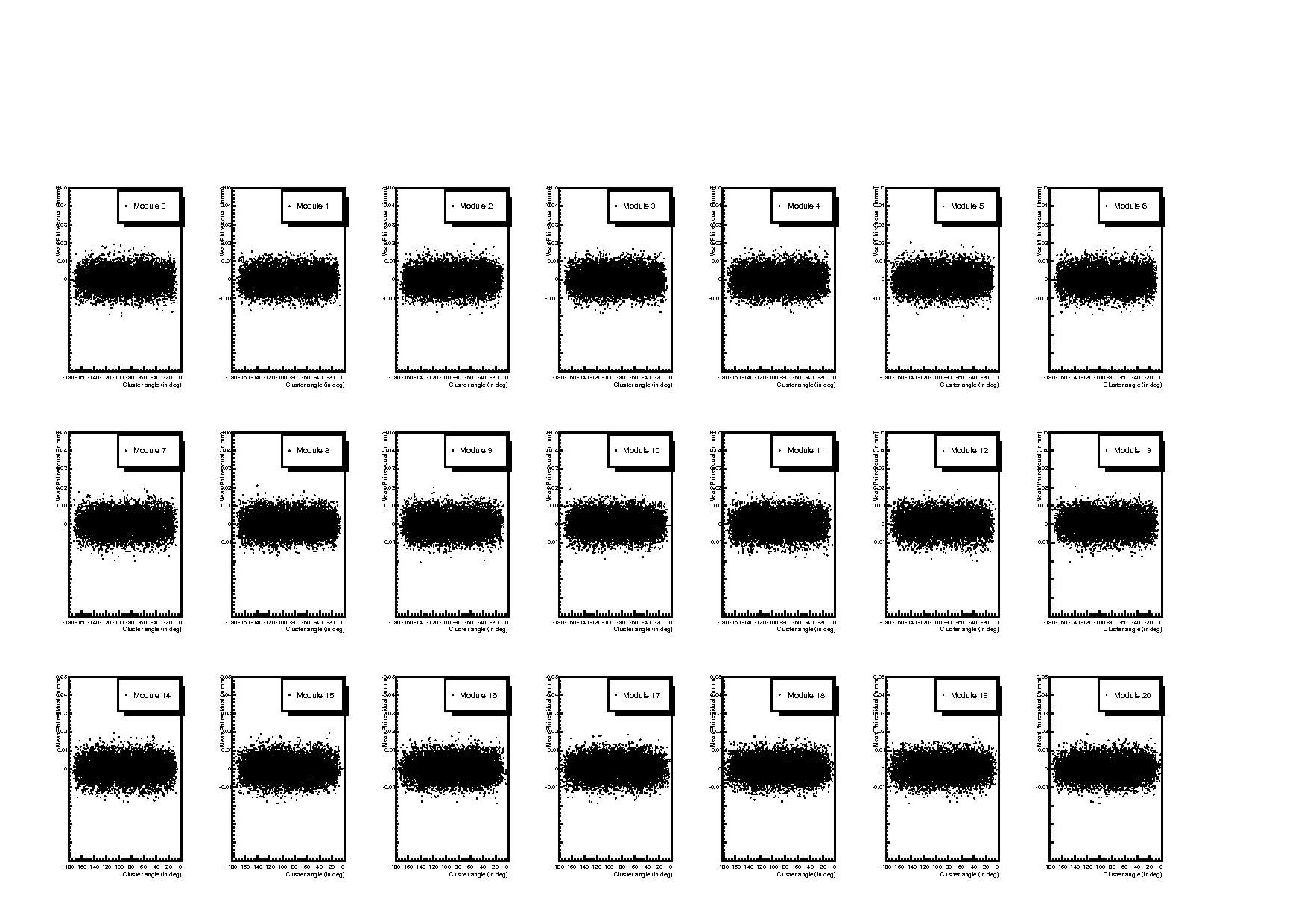
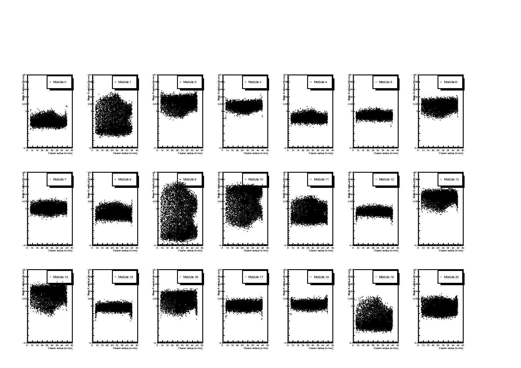
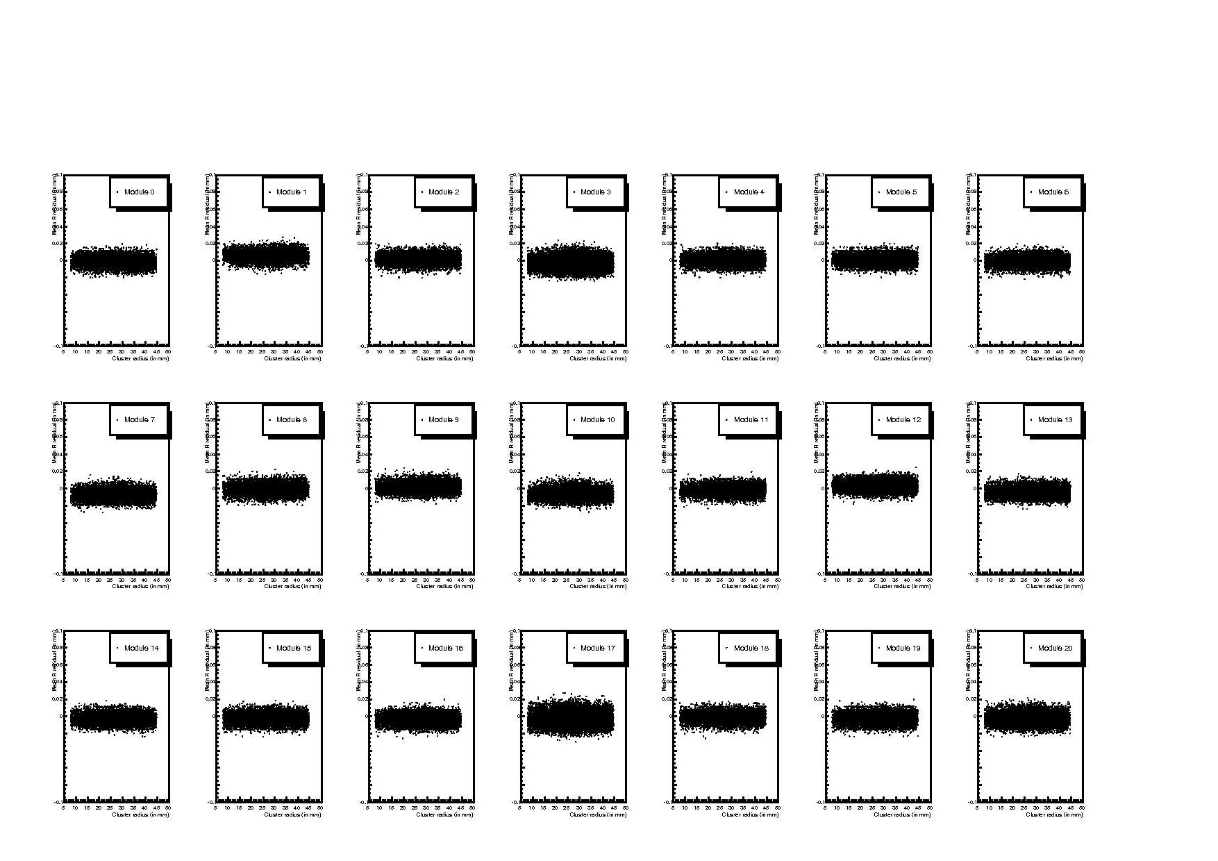
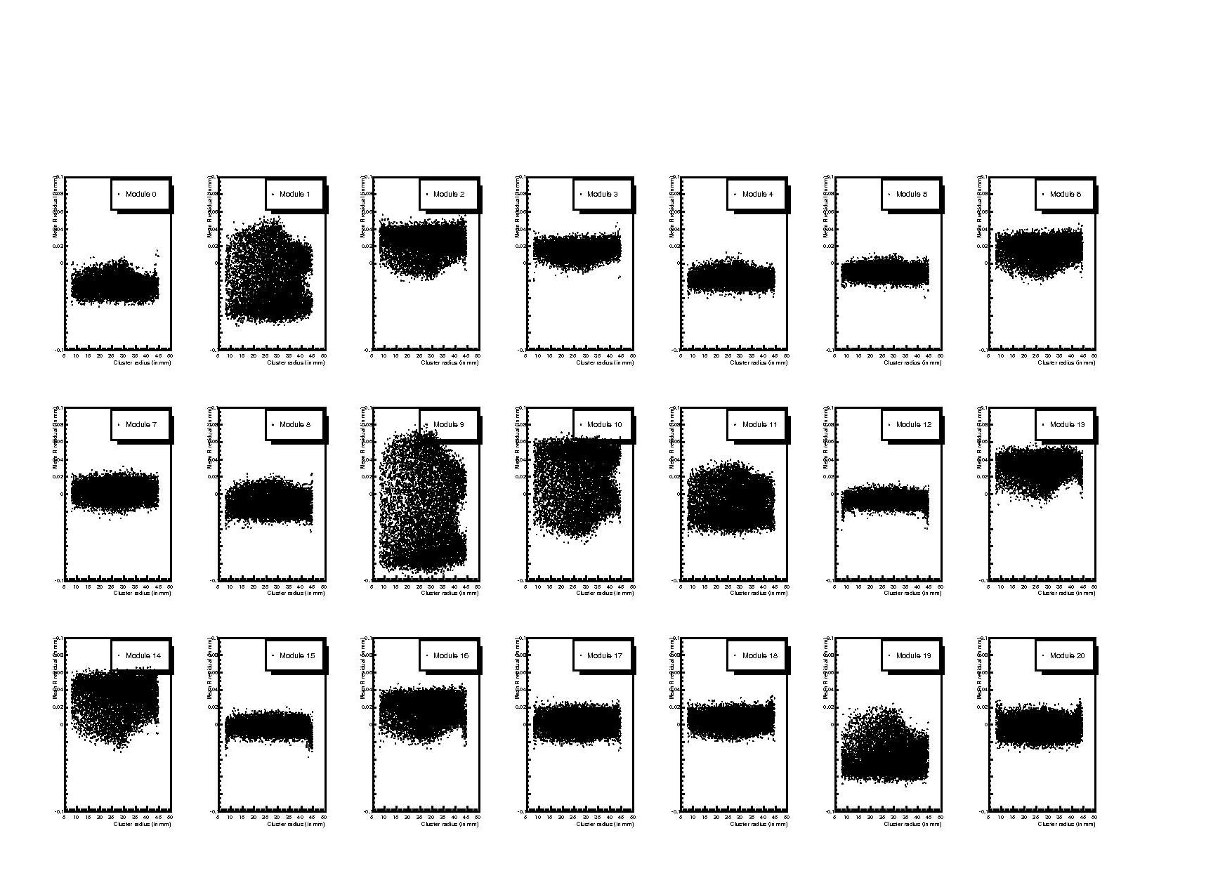
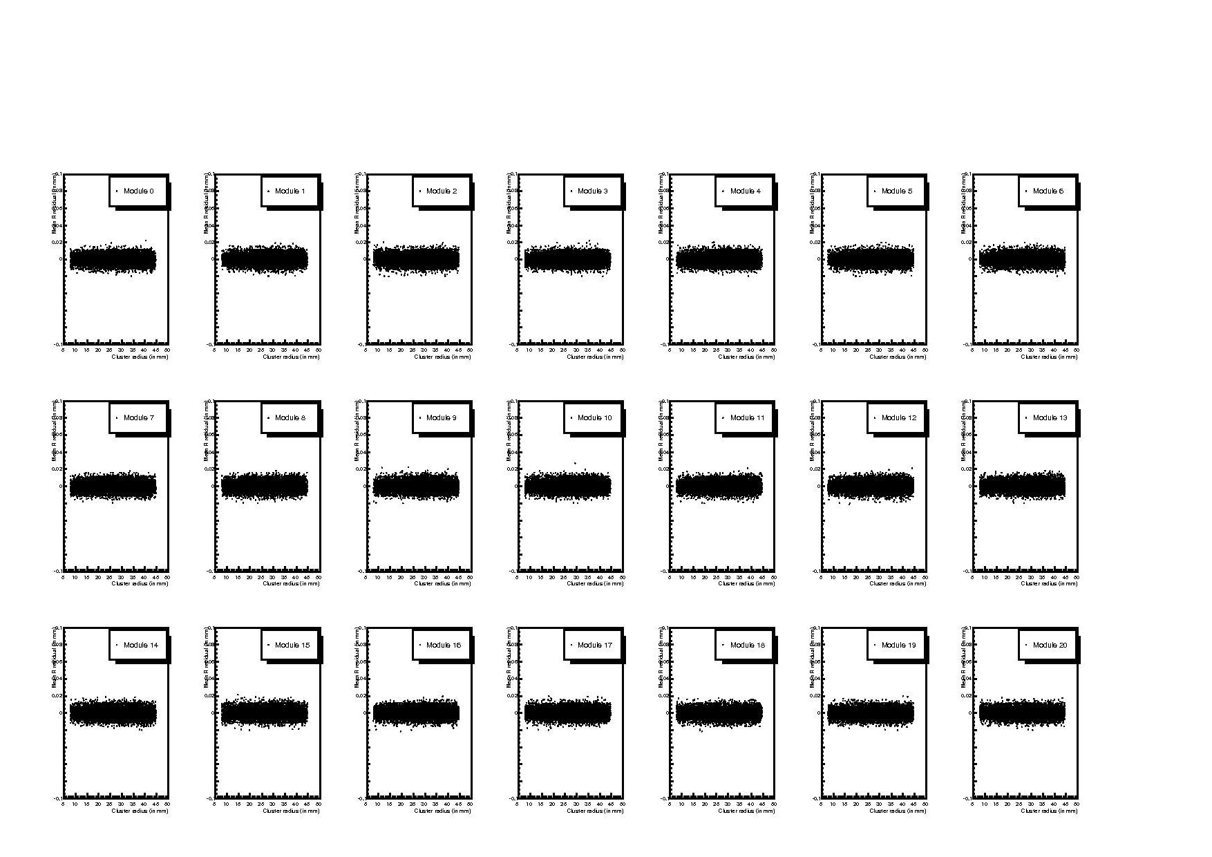
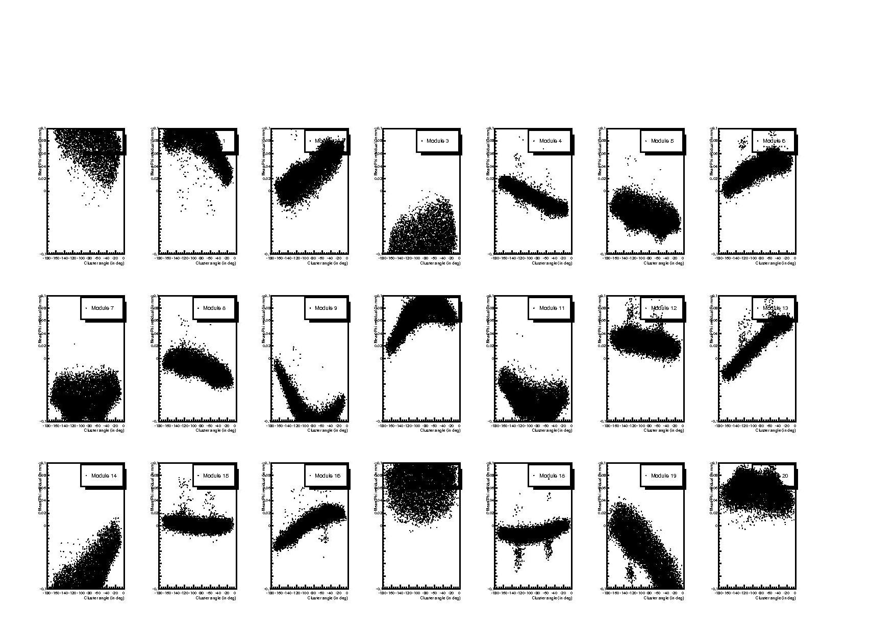
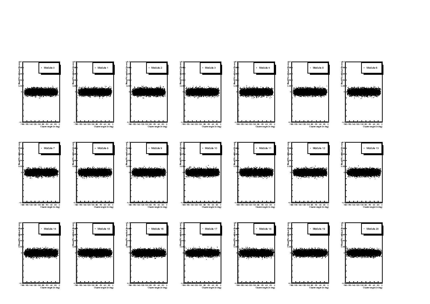
Each figure present the results for all 21 modules. The different sub-figures are defined as follows, from left to right:

Figure a : X space-points residuals before and after alignment (similar to the classic ACDC plot).
Figure b : Y space-points residuals before and after alignment.
Figure c : R cluster residuals, as a function of cluster radius, before alignment.
Figure d : R cluster residuals, as a function of cluster radius, after alignment.
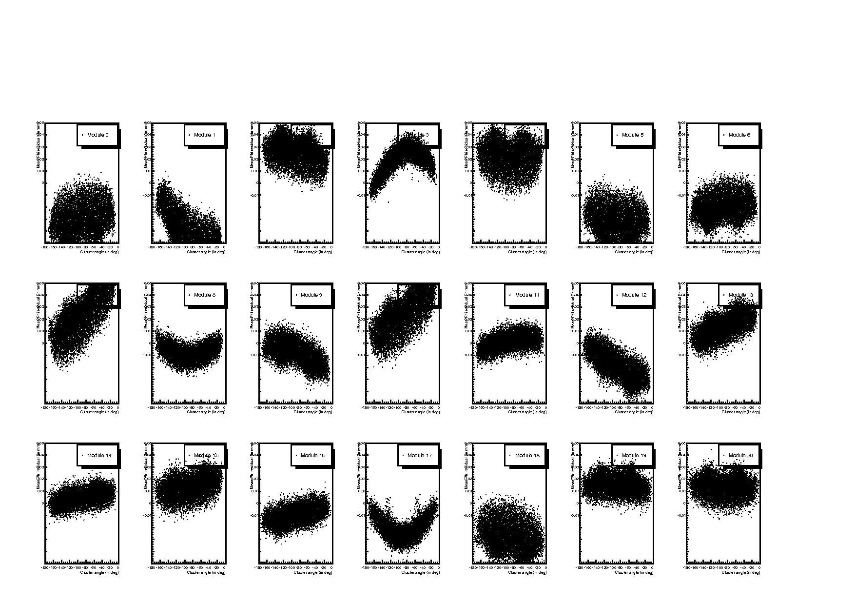
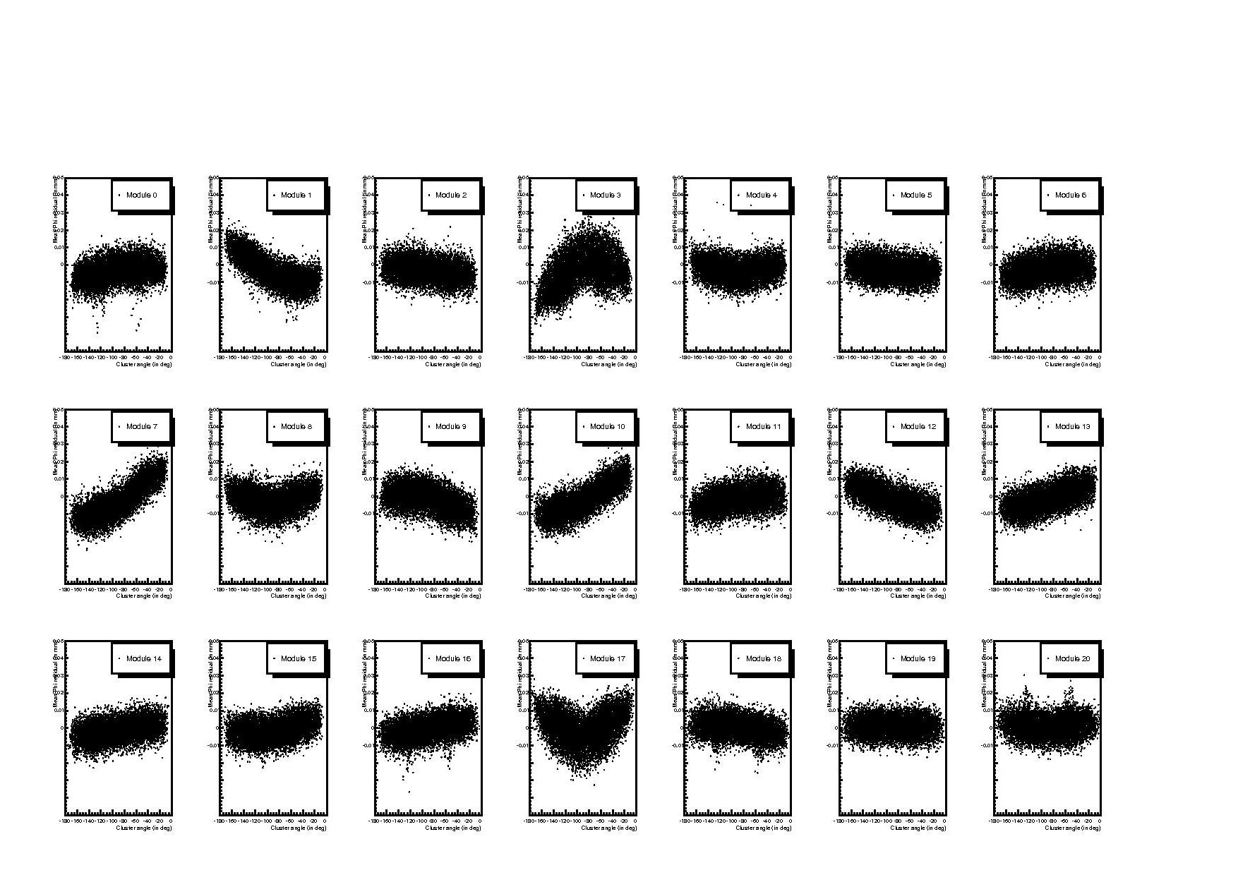
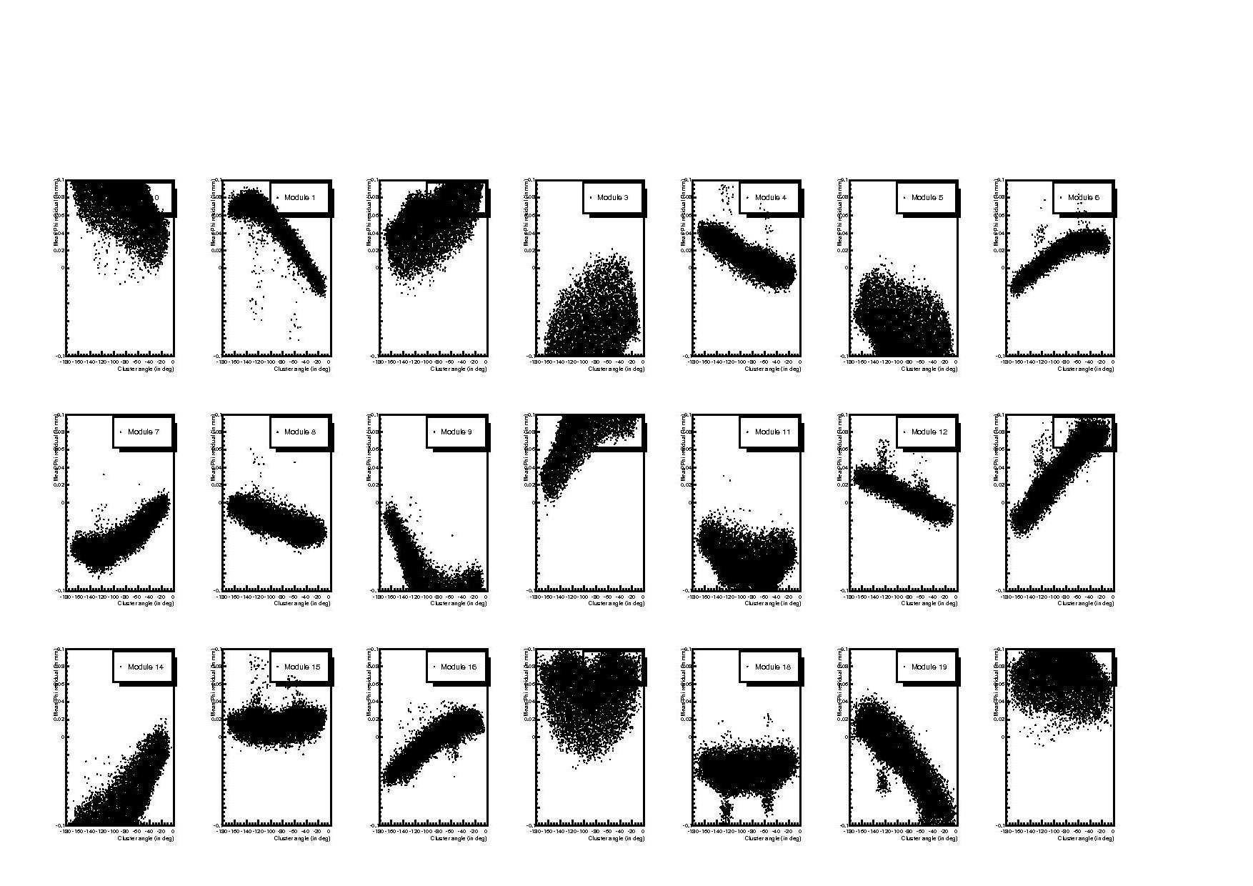
Figure e : Phi cluster residuals, as a function of cluster angle, before alignment.
Figure f : Phi cluster residuals, as a function of cluster angle, after alignment.

The first observation is that cluster residuals distribution, in particular with sensor misalignments, are quite similar to the one observed on the real ACDC3 data (in particular the Phi residuals 'banana' shapes). This means that the toy is not completely unrealistic and that we could grant some credit to those results.

The second point is that without survey information, residuals are still biased after alignment. But this biased could be clearly corrected if survey information is taken into account. This means that if the sensors didn't move after bonding on the hybrid, the survey should be fairly good and then gives us a good correction.

However, all this has to be confirmed via MC studies and with ACDC3 data.

C9. Sensor misalignments: A full MC study

C9.1 Introduction and method

A full MC simulation of the effect of misaligned sensors has been carried out.

The current Velo alignment algorithm uses only module misalignment constants as parameters. In this study, sensor misalignment constants were only used as geometry input, i.e. allowing for running the software with misaligned sensors, however the sensor misalignment constants were not treated as free parameters in the alignment algorithm. The aim of this study was to evaluate the influence of misaligned sensors on the current imlpementation of the alignment algorithm and thus their influence on module misalignment constants. Furthermore, this study should show the possible benefit of a detailed sensor survey for the quality of module misalignment.

The simulation was run on DC06 software (LHCb v21r12: Sim/Gauss/v25r7, Digi/Boole/v12r10, Rec/Brunel/v30r14). To introduce misalignment a private copy of Det/XmlConditions/v2r4 was used. In this one 10 sets of radnom misalignment constants were produced for each one of four misalignment configurations under study. The four configurations were (given are the scales for the random misalignments in mm for translations and in rad for rotations; A = alpha, B = beta, C = gamma):

module misalignment only (mod)
X,Y,Z = 0.03; A,B,C = 0.002
sensor misalignment only (sen)
X,Y = 0.01; Z = 0.1; A,B,C = 0
sensor misalignment only (sen2)
X,Y = 0.01; Z = 0.1; A,B,C = 0.001
sensor + module misalignment (senmod)
sen + mod

For each of these 40 sets 20000 particle gun events were produced, simulating pions with a momentum between 1 GeV/c and 100 GeV/c, evenly spread across the left half of the Velo and penetrating it as srtaight tracks (theta less than 0.005).

It is known from previous studies that the sensitivity on X, Y, and C is much better than that for Z, A, and B. Thus only X, Y, and C are taken as free parameters in the module alignment algorithm.

C9.2 Results

The first set of plots shows results from studying module misalignment only. The first three plots show resonstructed vs. generated module misalignment constants. Generated misalignment constants are the true inputs to the xml files. Reconstructed misalignment constants are those retrieved when running the alignment algorithm with a non-misaligned geometry. Ideally, both values should be the same, thus the distribution should show maximal correlation. The next three plots show the alignment resolution, i.e. the distribution of the difference of reconstructed minus generated misalignment. The resolution plot has been combined for the two translations. The retrieved resolution is 0.83(4) um and 0.134(8) mrad for translations and rotation, respectively.

The second set of plots shows results for the configuration with sensor misalignment (sen, no rotation) only. Again, the first three plots show reconstructed vs. generated module misalignment. The generated module misalignment constants are of course 0 as only sensor misalignment has been introduced. It should be noted that the case where both sensors were misaligned in the same direction, with respect to one of the misalignment constants, contains an intrinsic module misalignment. Or, the common part of the sensor misalignment is equivalent to a module misalignment. As this has not been taken into account as a generated misalignment, a certain part of the reconstructed non-zero module misalignment is due to this effect and thus 'real' module misalignment. However, as the situation that both sensors are misaligned in opposite directions happens equally often, it is estimated that more than half of the reconstructed module misalignment is due pure effects from misaligned sensors on the module alignment algorithm. Hence, the resolutions as shown in the last two plots clearly show an effect of misaligned sensors on the module misalignment constants. The obtained resolutions are 6.54(26) um and 0.265(14) mrad for translations and rotation, respectively.

In the third set of plots the results from the second configuration with sensor misalignment only (sen2, incl. rotation) are shown. Once more, three plots for reconstructed vs. generated module misalignment constants and two plots for the resultions. The resolution on the translations increased only slightly to now 7.80(35) um whereas the resolution on the rotation around the z axis increased significantly to 0.708(59) mrad. This is as expected as the difference to the previous case is only the introduction of random sensor misalignment in the rotation parameters.

The final set of plots shows the results for combined sensor and module misalignment (senmod). The sensor misalignment does not include rotations as described above (sen). Thus it is not surprising that, as the resolutions for module misalignment only were very small, the results are very close to those retrieved with sensor misalignment only (sen). The resolutions for combined misalignment are 7.23(30) um for translations and 0.334(19) mrad for rotation.

The results for the resolutions obtained with the different configurations are summarised in the following table.

	mod	sen	sen2	senmod
translation (um)	0.83(35)	6.54(26)	7.80(35)	7.23(30)
rotation (mrad)	0.134(8)	0.265(14)	0.708(59)	0.334(19)

An additional question tackled in this study was how those results compare to the intrinsic resolution of the alignment algorithm. This was estimated by running the alignment algorithm on the true misaligned geometry used to generate the events, i.e. the resulting misalignment constants should be exactly zero. This again was tested with all four configurations of misalignment constants. The follownig table shows the results for the intrinsic resolutions.

	mod	sen	sen2	senmod
translation (um)	0.17(0)	0.15(0)	0.17(0)	0.22(0)
rotation (mrad)	0.056(6)	0.028(3)	0.038(3)	0.049(6)

Two things should be noted here. Firstly, the intrinsic resolutions are much smaller than what is obtained in the more realistic case as studied above. Thus, the algorithm is able to produce acurate results and has no sognificant intrinsic bias. Secondly and more importantly, the intrinsic resolution is of the same size in all for cases. This means that an existing but well known sensor misalignment would not deteriorate the algorithm's ability to calculate the module misalignment constants.

C9.3 Outlook

It has been confirmed that the knowledge of the sensor misalignment is crucial to the module misalignment algorithm. The next step is now to apply the information from the sensor survey done in Liverpool to ACDC3 data and to test for a possible improvement in the alignment.

...Go to the next part...