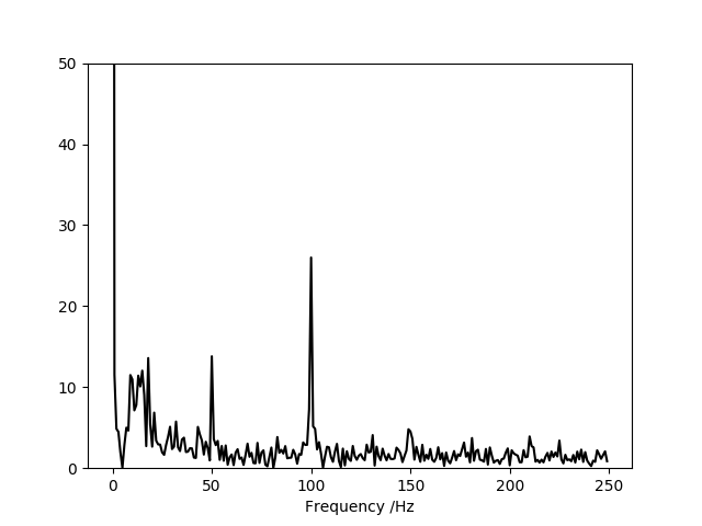
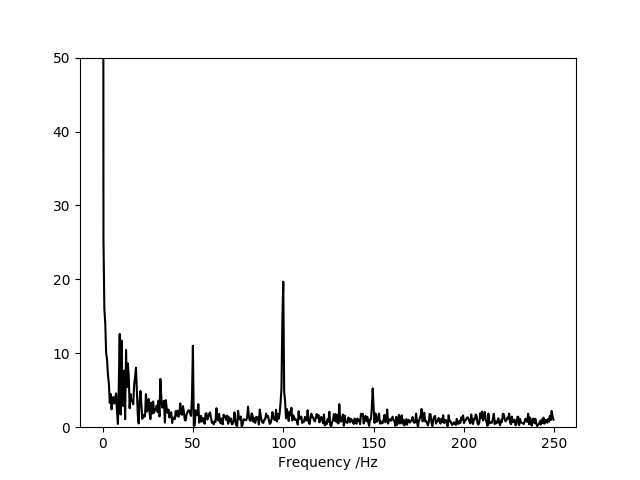
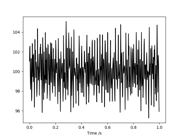
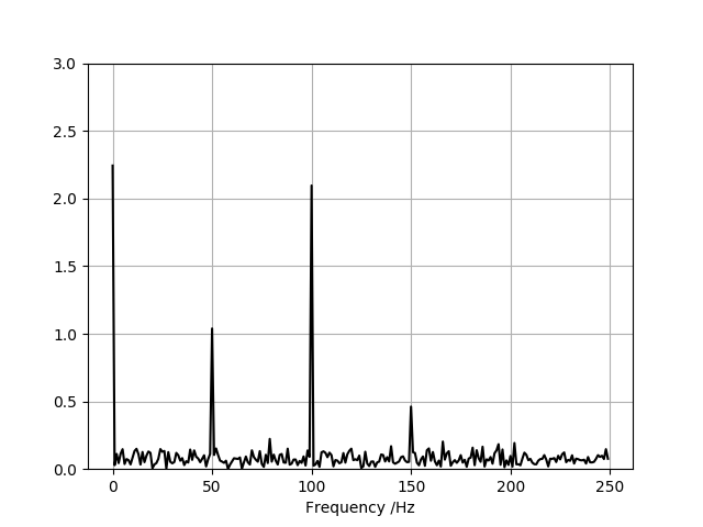
NA62 beam studies (23/3/23) (main plots from beam/html)
--------------------------

Time series analysis.
--------------------

The objective of a time series analysis is to determine the trend,
periodic, irregular and random components of the time series.
Here the time series is the rate of NA62 triggers taken
to be characteristic of the SPS spill.

Introduction.
------------

To illustrate some of the analysis techniques, a simulation of the spill and
and its analysis using Fourier transforms , periodograms
and difference plots is shown here

Fig 1 shows a simulation of the spill. A histogram of the number of events (triggers) per ms
is plotted over a one second period. 10**5 events are plotted. The trend is ~100 events per ms
and the random component is consequently ~10 events per ms.

In the simulation, sinusoidal components of 10, 50, 100 and 150 Hz have been
added to the trend with the 100 Hz present at the 10% level. The 10 Hz signal
has been added to illustrate the effect of a low frequency component (see the
autocorrelation plot). In addition, as frequently found in the data, there are
gaps in the spill; this has been simulated by the random addition of 25 1 ms
gaps in the spill. In reality, the length of these gaps varies. These gaps
constitute the irregular component of the time series.

Figure 2 shows two analyses that measure the periodic components of the histogram
of the spill. Figure 2a shows the sample autocorrelation. The dominant 100 Hz component
of the time series, modulated by the 10 Hz low frequency component, is clear.
Carefull inspection also indicates the influence of the 50 and 150 Hz signals.
A FFT analysis is shown in Fig. 2b. With the exception of the 150 Hz signal,
the Fourier transform separates the periodic parts of the spill fronm the background.

The same periodic analysis is repeated in Fig 3 using a periodogram and a Fourier transform
with a log axis that shows the zero frequency term measuring the total number of events
in Figure 1.
The periodogram confirms the results of the Fourier transform.

Figure 3 has two histogram showing the gross characteristics of the spill.
Fig. 3a plots a histogram of the size of the difference between two successive
bins of Fig. 1. This is, in effect, the first derivative of Fig 1 and should therefore
be a gaussian centered at zero with a width of sqrt(2*trend) in the absence of periodic
and irregular terms. Fig 3a shows that the periodic terms have only a small effect
on the gaussian peak. The irregular part of the spill forms tails about the peak;
consequently, the ratio RMS/Sigma is a good measure of the significance of the irregular component
of the spill.
Fig. 3b shows a histogram of the number of entries/ms of the spill. As would be
expected, the histogram is closely gaussian with a peak at trend and a width
larger than sqrt(trend) due to the periodic components. Any deviation from a uniform
trend will also increase the width of this distribution.
The irregular component appears as a separate peak at low counts for
the chosen form of simulation.

Data Analysis
-------------

The techniques discussed in the introduction have been applied to
nine bursts from the 2022 run. The sections below follow approximately
a sequence from low frequency millisecond general parameterisation of the spill
to spill chracaterisation in the microsecond range.

1) Frequency and first difference analysis.

The plots here show, for each burst,
in Fig.1 the spill histogrammed in 1 ms bins, followed in Fig 2 by the frequency
analysis of the spill in four one second time intervals.
Difference plots are given for the same time intervals in Fig. 3. In these
plots RMS refers to the root mean square(rms) of the histogram and
sigma to the rms of the gaussian fit to the central peak. The ratio, RMS/sigma,
is thus a measure of the significance of tails in the difference plots..
Finally, Fig. 4 shows, first, the difference plots for the 1.5 to 5.5 sec region
of the spill. As before, a gaussion distribution is fitted to the central
region of the distribution. The legend 'expected sigma' is, as explained
in the Introduction, sqrt(2*mean). The second plot in Fig. 4 is a histogram
of the number of entries per ms for the 1.5 to 5.5 second region of the spill
and shows clearly the irrecgular component of the spill when present..

The first burst analysed, 12567/336 , is typical of the majority of
the bursts in the sequence presented here: the periodic frequency 100 Hz
is dominant, 50 Hz is present over part of the spill, and an irregular term
is present in the middle of the spill. There is also low frequency 'noise'
present which is largest in the center of the spill and consequently may
result from irregular gaps in the spill.

The final burst in this list, 12066/1129, has no irregular component.
Consequently, there are no tails to the first difference distrubution and
RMS/sigma ~ 1.0 . The spill distribution, however, does not have the
expected sigma, sqrt(mean), since the trend of the spill is not flat.

2) High frequency spill characteristics.

The plots to be discussed in this Section
show the high frequency characterists of the spill that result, in part, from
the 5 x 2 structure of the SPS fill.

Fig. 1 shows the time structure of the spill in 5 ms bins, with Fig. 2 showing
the same distrution in 0.2 bins to illustrate the fine structure.
The large-scale characteristics are tabulated in Fig. 3 together with a histogram
of the number of triggers per ms. Typically, Fig 3 shows that the spill
has negative skewness due to the gaps in the spill, kurtosis greater than the 3
expected for a gaussian distribution, and a mean number of triggers/ms ~ 100.
Bursts such as 12066/1129, that have no irregular term, tend to have a positive
skewness due to the periodic component..
Fig. 4 demonstrates the spill structure that results from the SPS.
Here is plotted the spill trigger time (ms) vs the trigger time in 25 ns bins modulo 923.99xx
(the 'folded time').
The 923.99xx term ( the fold time) is found by minimizing the signal in the gaps in the projection of the
spill time on the folded time axis after correcting the folded time. The correction
to the folded time used is 2.4*(spill_time -1.5)**3 in folded time units with spill time in secs.
This correcion partially removes the effect of the reduction in momentum of the
beam as it circulates the SPS.
The corrected spill vs folded time is shown in Fig 5. Three projections
on the folded time axis are shown in Fig. 6 to illustrate the influence of the correction
and the fine structure of the beam. These two Figures suggest that the beam is rarely
fully debunched and that, especially at the start of the spill, there can be substantial
variations in intensity in a bunch.
Figure 7 has autocorrelation plots for folded time (7a) and spill time (7b).
Fig 7a has a peak at zero time lag showing a strong correlation over short time intervals.
Other peaks correspond to the bunch structure. Fig. 7b shows the dominant 50 Hz
or 100 Hz periodic term in the time series of triggers that is often modulated by a
low freqency component of the spill.
Figures 8a and b illustrate a section of the spill and its associated Fourieer analysis
indicating the dominant low frequency periodic components of the trigger times.x.

3) Time difference analysis

Histograms of the interval in time between succesive triggers are shown here
These plots illustrate the higher frequency components of the spill originating from the SPS..
The first three Figures show the general spill characteristics: firstly, a histogram af the spill
in 1 ms bins; secondly, a smoothed histograms of the spill to indicate the dominant periodicity
and, thirdly, a histogram of the number of entries per bin in the first histogram to give the mean
and rms of the trend of the spill.
Figure 4 is a log plot of a histogram of the time between triggers in microsecond bins.
As expected for a Poisson distribution this is a straight line with slope ~0.1 events/musec.
Deviations from the straight line are evident at half the circuation period of the SPS.
Figure 5 reapeats this plot over a wider range of time intervals. The majority
of bursts have peaks at ~ 0.2 and 0.33 ms. that are probably the irregular terms in the spill.
Finally, Figure 6 repeats Figure 5 with a plot of the difference between the histogram
of time differences and the ftted line. The plot again shows evidence for the 5 X 2
bunch structure of the SPS beam.

--------------------------------------------------------------------------------------------------------------
kspill versions - mainly high frequency

SPILL - poisson plots - time interval plots

Fig 6d kspill6.kumac . High frequencyTime interval plots.
new plots P1 for mean/variance + sample variance (20/2/23)
3/3/23 9 files gaussian for 1 ms limited range fit. prob gaussian.
*Main version*.

Fig 6dev kspill6dev.kumac . High frequencyTime interval plots.
Dev version of kspill6.kumac. Check spillassociated with gaps. 100523 -

Fig 6g kspillff.kumac to kspillf.ps (pdf) for filter tests.
3/3/23 version: filter tests for 100 ms and 1 sec. Demonstrates effect of filtering
and shows the low frequency component.

Fig 6h kspillp.kumac , test periodogram 1 sec (kspillff derivative)

Fig 6h kspillp2.kumac , test periodogram + correlogram (kspillff derivative)

Fig 6h kspillp4m.kumac , test periodogram * 4 (4 secs) (kspillff derivative)
Displays kspillp4m.kumac outputs kspillp4.pdf , uses modified periodogram that dispays amplitude( equiv autocorr10m.kumac)
Difference plots, spill gaussian comparison. First/Second difference plots added 06/04/23
Note 2nd diff plot gives central rms fit = sqrt(6.*mean)
*Main version*.

Fig 6h9 kspillp4m9.kumac
Single set of plots for final spill 12066/1129 additional difference plots with lags. 110423 .
Updated 17/4/23 . Copied to ab2.kumac for optimisation and further development.

************************************************************************************************
************************************************************************************************
************************************************************************************************

Fig 6ab2 ab2.kumac . Reorganised version of kspillp4m9.kumac
2 files

Fig 1 Spill distribution
Fig 2 Difference plots: the cyan lines show two stanard deviation limits expected from statistical errors.
These plots are insensive to low frequency periodic signals but indicate irregular noise terms
in the spill.
Fig 3 Periodograms showing periodic noise frequencies.
Fig 4 Difference plots. The central peak has width defined by statistical noise. The tails of
the distribution are due to rregular noise.
Fig 5 Spill distribution: the Gaussian peak has a width due to statistical and periodic noise.
The small peak at ~ 20 is due to irregular gaps in the spill.

Fig 6ab2all ab2all.kumac . All files - as ab2

Fig 6ab19 ab19.kumac . extra 2nd diff plot All files

Fig 6ab22 ab22.kumac . single plots

Fig 6ab2dev ab2dev.kumac . Reorganised version of kspillp4m9.kumac
dev version

Fig burst2 burst2.kumac . Reorganised version of ab2.kumac
Skewness, kurtosis added. Produces fort.33 , burst2.output.

burst2.kumac burst2.kumac . code . output to fort.33, burst2.output.
run,burst,ratio,skew,error_skew,kurtosis

Fig burst2dev burst2dev.kumac . histo fit via hbook - test

burst2dev.kumac burst2.kumac . code . output to fort.33, burst2.output.
Anotated, has HBOOK Gaussian fits see Figs. 4 and 5 that could replace the PAW fits.
version 290423 ie burst2dev.kumac.290423 is backup - 1 ms plots. Subsequently updated .5 ms.

Fig burst3dev burst32dev.kumac . Simplified plots
0.5 ms only shown. Spill + first diff plots. Goodness of spill defined by RMS of first diff.
This pdf file is produced by burst32dev.kumac 030523. Produces fort.44

Fig burst32dev burst32dev.kumac . Simplified plots. 12/05/23
pdf is from burst32dev.kumac 12/05/32. 3 new files 10-12.

Fig burst3dev.kumac burst32dev.kumac . code . 0.5 ms

Fig fort.44 fort.44 test file Dump of Alan's data.

--------------------------------------------------------------------------------------------------------------

AUTOCORR versions - general beam parameters - high frequency + low frequency.

Fig 11g autocorr10m.kumac - FFT minimal version
Updated to display autocorr10m.kumac FFT with trend subtracted. (o/p to autocorr10.pdf) 04/03/23
*Main version*

Fig 11h autocorr11.kumac - FFT for 1 sec spill regions.

*************************************************************************************************
Fig 11dev autocorr10dev.kumac as autocorr10m.kumac + 12 files -frozen
26/7/23 see p 92 for the effect of 100 Hz 14000 amplitude signal on spill intensity distribution.
Factor 6 range of intensity.
************************************************************************************************

Fig 11dev2 autocorr10dev2.kumac dev version

--------------------------------------------------------------------------------------------------------------
--------------------------------------------------------------------------------------------------------------
--------------------------------------------------------------------------------------------------------------
--------------------------------------------------------------------------------------------------------------
--------------------------------------------------------------------------------------------------------------

New code for 23 data and spill statistics plots
----------------------------------------------

Fig 1 burst231.kumac for 2023 data developed from kspill6dev.kumac
Add periodogram, folded distrubutions.

Fig 2 spill statistics 22/23 spillstat.pdf

Fig 3 spill statistics 22/23 file spillstat.f

Fig 4 spill statistics 22/23 files,spillstat.kumac

Fig 5 spill statistics 22/23 periodogran added for noise measurement

Fig 6 spill statistics 22/23 periodogran added for noise measurement
plus folded spill plots for uncorrected data, spill in 5 ms bins, RMS plots.
code: spillstat3.f ,
spillstat3.kumac"
Fig 6 now shows output from spillsta4.kumac, if this has been run last since this outputs spillstat3.ps.

NOTE: spillstat4.f spillstat4.kumac have autcorrelation plots (correlograms) in addition to
those in spillstsat3.f, .kumac. The files produced are spillstat3.dat , spillstat3.ps ,spillstat3.pdf ;
./clg75 spillstat4 spillstat4 , ./spillstat4 , PAW exec spillstat4 , convert spillstat3.ps spillstat3.pdf,
cp spillstat3.pdf public_html/newplots .

Fig 7 spill4.kumac . reordered event by event from spillstat4.kumac.

Fig 7dev spillistat5.kumac . reordered event by event from spillstat5.f.
dev. version

Fig 8 kstat4.kumac . As spillstat4.f plus spill4.kumac but is a
single kumac containing spillstat4 as a subroutine and the PAW section of spill4.kumac.

Fig 9 kstat4a.kumac . As spillstat4.f plus spillstat4.kumac but is a
single kumac containing spillstat4 as a subroutine and the PAW section of spillstat4.kumac.

Fig 10 kstat4adev.kumac as kstat4a . dev version - annotated

Fig 11 kstat4adev.kumac code

Fig 12 kstat44.kumac 1 plot/burst: spill, folded spill, freq, autocorrelation.

Fig 12a kstat44a.kumac 1 plot/burst: spill, folded spill, freq, autocorrelation.
alternative organisation.

Fig 12adev kstat44adev.kumac 1 plot/burst: spill, folded spill, freq,
autocorrelation. New .txt files with nhits. hits plots with skewness,kurtosis.

Fig 12adev2 kstat44adev.kumac 1 plot/burst: spill, folded spill, freq,
autocorrelation. New .txt files with nhits. hits plots with skewness,kurtosis.
Frozen - 8 figs including hit plots. 130623.
------

Fig 12dev kstat44dev.kumac 1 plot/burst: spill, folded spill, freq, autocorrelation.
dev version: added analysis of folded spill, autocorrelation. 2nd plot. In progress.

Fig kdev1 kdev1.kumac 1 plot/burst: spill, folded spill, freq, autocorrelation.
Derived from kstat44adev2.kumac. New text files. Dev version 130623. Keep as a stable version. add back noise,
combine figs 7 and 8. align folded spill vs hits ( approx time). Freeze - best version to date (13/06/23 ).
-----------------------------------------

Fig kdev2 kdev2.kumac as kdev1.kumac . dev version. from 130623 dev1.kumac
Version with indicated poor spills in Figs. Freeze 16/06/23.
Fig kdev2code kdev2.kumac code 16/06/23§

Fig kdev3 kdev3.kumac as kdev2.kumac . dev version. from 160623 dev2.kumac
keep as standard 23/6/23

Fig kdev4 kdev4.kumac as kdev3.kumac . dev version. started 23/6/23
with hit cut 125, cutb on fig 1 set at 10. keep as updated standard to minimise effect of high beam intensity.

Fig kdev5 kdev5.kumac as kdev4.kumac . dev version. started 24/6/23
for further hit cut development. Print/display of % data removed - otherwise as kdev4.kumac

Fig kdev51 kdev51.kumac as kdev5.kumac . dev version. started 24/6/23
for further hit cut development. Main dev version - hits reordered, plots reordered. .
No memory space to store folded times in kumac but hits reordered as in spill , folded spill. code saved on mac.

Fig kdev51code kdev51.kumac code 250623 . reodered hits, plot order changed.
displays number of triggers removed in Fig 1. Fig 1 has triggers removed , title shows cuts.
Fig 3 plots folded distr. with triggers removed; all other Figs. unchanged. Best version of code to date

Fig kdev52 kdev52.kumac as kdev51.kumac . 26/6/23
Version for major changes on hit removal. hit removal coded, see ' go to 123 , 123 continue ' and removed
because majority of high hit level is not removed by cuts on the spill-filled spill 2D plot.

2023 DATA

2023 DATA 85 Bursts received 28/06/23

Fig kdev511 kdev51.kumac run on 23 data 29/06/23 new files from Alan
files in ~/afile . Bunch count. Bad bursts selected. KEEP - STANDARD. This is latest version
of bunch count and is the basis for a fortran version. 020723 is standard - pro tem.

Fig kdev511code kdev511.kumac code 02/07/23

Fig kdev512 kdev51.kumac run on 23 data 29/06/23 new files from Alan
files 1 - 85 . All events run - no selections. KEEP - STANDARD. No bunch count but otherwise
similar to kdev511.kumac.

Fig kdev55 kdev55.kumac run on 23 data 28/06/23 new files from Alan
from kdev512.kumac. Version run for high frequency studies of bunch structure. Dev. version.
Bunch count - old version.

Fig kdev551 kdev55.kumac run on 23 data 28/06/23 new files from Alan
from kdev512.kumac. Version run for high frequency studies of bunch structure. Alternative Dev. version.
Bunch count - latest version - used in kdev511.

Run 13340 140 bursts received 04/07/23
---------------------------------------

A) kumac based analysis ( BQI - Burst Quality Indicator)

Fig kdev340 kdev340.kumac (copy of kdev511.kumac)
10 events test.

Fig kdev341 kdev340.kumac (copy of kdev511.kumac) BQI set.
Plots selected BQI events ( output from kdev340.kumac is to kdev341.ps converted to kdev341.pdf)
extra plot hits/triggers 15/07/23.

Fig kdev340all kdev340all.kumac . ALL BGI sel. events
extra plot of hits/triggers 15/07/23 and hits vs spill time + MAX/MIN etc

Fig khit1 khit1.kumac from kdev340all.kumac for hit analysis
and development) 230723. BQI plots for skewnees, %excess at end.

Comments: Fig 9b shows the effect of dead-time: at the start of the spill a high intensity spike
does not result in an equivalent number of triggers due to dead-time effects.
Consequently, beam intensity is better measured using GTK(1) hits rather than triggers.

The skewness of the hit distribution, Figs. 8a and b, Plot 400, is a good indicator of
spikes in the distribution and hence possible overloading of the readout system. Plot 400
shows a tail to the distribution that indicates significant spikes in a few bursts.

These spikes may be of high intensity but short duration. A measure of the overall importance of
these high intensity regions can be defined as

BQI %excess = 100* (number hits greater than 1.5* mean)/(total number of hits in burst),
see plot 410. This plot suggests a tail to the distribution of this BQI but that there
are few bad bursts based on this criterion.
(The 1.5 factor correspond to ~ 4sd. statistical error).

--------------------------------------------------
Fig khit2 khit2.kumac - stable version - 02/08/23
Version with high intensity regions marked in cyan

Fig khit2mod khit2mod.kumac - stable version - 07/02/24
For two-page plots

Fig khit2modp khit2modp.kumac - burst 1211 -15/03/24 for paper

Fig khit2modpp khit2modpp.kumac - burst 1211 -18/03/24 has additional profile plot to illustrate the difference
between GTK1 hits and triggers. profile plot removed

Fig khit2modpp2 khit2modpp2.kumac - burst 1211 -18/03/24 has additional profile plot to illustrate the difference
between GTK1 hits and triggers. Try improving profile plot.

--------------------------------------------------

Fig khit3 khit3.kumac -stable version 23/08/23

Fig khit3all khit3.kumac dev. version 06/08/23 all events

Fig khit4 khit4.kumac - with hit/ trigger lt 100 cut 27/08/23
(This and khit3 have no space left for additional code)

Fig khit5 khit5.kumac - dev version (code removed) 27/08/23

**********************************************************************************

Fig khit51 khit51.kumac 1/11/2023

STANDARD VERSION for LOW FREQUENCY ( ~ ms ) ANALYSIS
BQI set.

**********************************************************************************

Fig khit5110 khit5110.kumac - dev version - 'extreme tests' 110923
110 hit cut applied - compare khit51.kumac
Used for tests of gt and lt 50 hits (12/09/23).
No BQI signals for lt 50 hits in GTK1.

Now reset to gt 110 hits rejected - this results in all 'spikes' BQI being removed
and only 100Hz and 'Excess' BQI being set.

Fig khit51h khit51h.kumac - dev version - high intensity
All events after 110 hit cut.

Fig khit51hh khit51hh.kumac - dev version - high intensity
For high frequency.

Conclusions (24/09/23)
-----------

1) The GTK(1) hit distribution associated with triggers is closely Gaussian with mean ~ 50 hits and width 15 hits.

2) There is a non-Gaussian tail to the hit distribution with ~ 1 in 1000 triggers having more than 110 hits in GTK(1).

3) The triggers associated with more than 110 hits in GTK(1) give rise to peaks in the distributions
of the spill and/or folded spill.

4) THe RMS of the GTK(1) hit distribution is a factor ~ 2 greater than that expected from the mean of the
distribution. Tha results presented here suggest that this is due to the 50 and 100 Hz resonances
and the low frequency noise displayed in the Fourier analysis of the spill,

Comments 3/11/23
-----------------

khit51.kumac: latest version 1/11/23.
khit3.kumac: has additional plots that dispay the folded hit distrbution.

B) fortran based code

Fig fkdev340 fkdev340.kumac (o/p from fkdev340.f)
Plots distribution of variables used as BQI.

Fig fkdev340f fkdev340f.kumac single burst test.
fkded340f.f outputs a set of BQI selected events (6 in this 140 set of bursts.
Plots spill, folded spill, Hz , autocorrelation, hit distributions as kdev340.kumac.
Burst 1211 shown here.

C) Fortran code

code Program reads data, sets up hbook,
subroutine - input via common (kstore, hstore) - evaluates BQI -
single file for each burst with bad BQI. Derivative of fkdev340f.f (Section B).

FFT tests

Fig Ea fftplot1dev.f to cft1.kumac - FT stand-alone - cft version -file 1
Fig Eb fftplot2dev.f to cft2.kumac - FT stand-alone - cft version -file 2
Fig Ec fftplot3dev.f to cft3.kumac - FT stand-alone - cft version -file 3

Fig E1 fftplot41.f to cft41.kumac - FT stand-alone - cft version -file 1
Fig E2 fftplot42.f to cft42.kumac - FT stand-alone - cft version -file 2
Fig E3 fftplot43.f to cft43.kumac - FT stand-alone - cft version -file 3

Fig Ed fft1test.f to cft1test.kumac - FFT stand-alone - cft version -file 1
test version
Fig Ed fft2test.f to cft2test.kumac - FFT stand-alone - cft version -file 2
test version
Fig Ed fft1test.f to cft3test.kumac - FFT stand-alone - cft version -file 3
test version

-------------------------------------------------------------------------------------------------------------

SPILL SIMULATION for comparison with data. Low ftrequency.

Simulation FFT periodogram , difference plots

Fig 122 simulation, corrtest22m.kumac - check autocorr , FFT, standard
periodogram. Set to show output from corrtest22m.kumac.

corrtest22m.kumac FFT + modified periodogram for f = 0 and amplitude.
corrtest22m.kumac to corrtest22.ps mod to give same results as FFT (09/03/2023 ). Use this version for tests.

Demonstrates:

Peak at f = 0, = number of input events
Peaks at f .ne. 0, = (0.5 * amplitude) of sin/cos terms.

Set to show 100Hz ( k = 5 )

Fig 12dd simulation of data, corrtestdd.kumac. structure as corrtest22m.kumac
100 events/ms. 10**5 events in total. 10% 100 Hz signal + 10 , 50, 150 Hz terms. 10 Hz to
Indicate effect of low frequency 'noise'. Similar to 12066/1129 for 50, 100 150 Hz signals.
*Main version*.

Fig 12dd2 simulation of data, corrtestdd2.kumac. Dev. version.
Add gaps to simulate data gaps. Results as expected: bg raised, tails to difference plot produced.
Compare with corrtestdd.kumac.
*Main version.

Fig 12nn simulation of noise, corrtestnn.kumac.
*Main version*.

Fig 12dev corrtestdev.kumac.
* dev/test version*.

Fig 12nndev corrtestnndev.kumac.
Has check of difference equation y(t) = a1*y(t-1) +a2*y(t-2) a1 = 1.617 a2 = -1.0
gives 100Hz if 1 interval in time = 1ms. see plot 8500
* dev/test version*.

Fig 12nndev2 corrtestnndev2.kumac. with time difference plots
to check kspill6.kumac. verifies sort - but events produced by uniform time distribution.
Has simulation of poisson distribution in two forms.
* dev/test version*

Fig 12dev4 corrtestdev4.kumac. Yet another dev version
for systematic studies. from corrtestnndev2.kumac
Add (11/04/23) : 50 Hz + difference plots with different lags to show increase in sigma.

Fig alan1 alan1.kumac - plots - version of corrtestdd2.kumac
Fig alan1.kumac alan1.kumac - code - version of corrtestdd2.kumac

corrtest2d simulation 2D separable function

corrtest2ddev.kumac simulation 2D dev

corrtest2df.kumac simulation 2D from corrtest2df.kumac reading
output from corrtest2df.f (corrtest2df.dat to corrtest2df.ps )

Fourier Transform - Python code

Fig 6 Fourier transform of spill (3 - 4 sec) 12465/170

Fig 7 Fourier transform of spill (3- 5 sec) 12465/170

Fig 8 simulate 50, 100, 160 Hz spectrum (fftcode1.py ) 30/11/22

Fig 9 Fourier transform of simulation fig 8 (fftcode1.py) 30/11/22

BQI plots 4/2/2024

Fig1 Test plots

Fig2 Test plots all events rdatha1.f run 12567
(replaces rdatha.f .kumac)

Fig2s rdatha1.f to bp1.kumac (short rdatha1.kumac) run 12567
----------------------------------------------------------------------------------------------

Fig2a Test plots all events rdatha2.f run 13662

Fig2b Test plots all events rdatha3.f run 12288

Fig2bs rdatha3.f to bp3.kumac (short rdatha3.kumac) run 12288
-----------------------------------------------------------------------------------------------

Fig2c Test plots all events rdatha4.f run 12165

Fig3 run 12567 khit51bqi.kumac

FigA 3 plots for Alan

BQI_notes BQI notes 08/02/2024

_Spill Duty Factor SDF notes 28/02/2024

BQI writeup_ BQI notes 21/03/2024

BQI writeup_version 2 BQI notes version 2 9/04/2024

Time difference plots time difference plots ns 22/04/24 - short version-standard
L0 L1 plot kspill61.kumac

Time difference plots time difference plots ns etc 07/05/24
L0L1 plots and more kspill61dev.kumac

Time difference plots time difference plots ns etc 21/05/24
L0L1 plots and more kspill61devh.kumac 2023 data

BQI plots 2024 for studies of quality cuts

BQI distributions mean RMS and SDF distributions: spill624.kumac
from spill624.f.

BQI distributions mean RMS and SDF distributions: spill624a.kumac
from spill624a.f. As above but files from skilli-bqi/eosfiles2/014160 - 014163

BQI distributions mean RMS and SDF distributions: spill624b.kumac
from spill624b.f. As above but files from skilli-bqi/eosfiles2/014170 - 014182

*********************************************************************************************************************
*********************************************************************************************************************
****************** main BQI studies - cuts, correlations 2024 data *************************************************** 11/07/24

BQI distributions mean RMS and SDF distributions: spill624c.kumac
from spill624c.f. As above but files from skilli-bqi/eosfiles2/014160 - 014182 (updated spill624b)
Comment: a set of runs with no significant 2 sec spike, see Fig. 6 . Figs 7a, 7b for 2sd cuts.

BQI distributions mean RMS and SDF distributions: spill624d.kumac
from spill624d.f. As above but files from skilli-bqi/eosfiles3/014201 - 014212
Comment: a set of runs with the 2 sec spike present, see Fig. 6. Figs. 34 a, b illustrated SDF for good/bad runs.
Fig 35c shows effect of removal of spike on Fig. 34b.

BQI distributions mean RMS and SDF distributions: spill624e.kumac
from spill624e.f. As above but files from skilli-bqi/eosfiles3/014238 - 014275
Spike at start of spill + some 2sec spike.

*................................................................................................................
* SHORT VERSION with pdf from spill624ds2.kumac (input from spill624d.f)
BQI distributions mean RMS and SDF distributions: spill624ds.kumac
from spill624d.f. As above but files from skilli-bqi/eosfiles3/014201 - 014212 . SHORT VERSION.
Figs. 33 - 35
NOTE: plots here are from spill624ds2.kumac. Thes have mean and sd of the SDF and normalised RMS. nRMS favoured as diagnostic because it showes a larger
% change between 'good' and 'bad' runs 14212 and 14202, respectively.
NOTE:
spill624ds2.kumac reads output from spill624d.f.
spill624ds2.kumac prduces spill624ds.pdf
spill624d.f -> spill624d.dat -> spill624ds2.kumac -> spill624ds.ps -> ./trans spill624ds -> spill624ds.pdf
*................................................................................................................

*................................................................................................................
SHORT version of spill624e
BQI distributions mean RMS and SDF distributions: spill624es.kumac
from spill624e.f. SHORT version of spill624e.kumac. As above but files from skilli-bqi/eosfiles4/014238 - 014275
Spike at start of spill (1.5ms) + some 2sec spike

Updated version: 30/07/24.
spill624e2.f produces spill624e2.dat as input to spill624es2.kumac that produces spill624es.ps
use ./trans spill624es to sipp624es.pdf. This version has plot 1583 - % of nRMS gt 2.5 .
.
*................................................................................................................

source setcd
/data/na62_01/skilli-bqi

./clg75 spill624d spill624d
paw exec spill624d
./trans spill624d

**************************************************************************************************************
*********************************************************************************************************************
*********************************************************************************************************************

BQI distributions MEAN, RMS, SDF and RMS/sqrt(MEAN) distributions: spill6244.kumac
Input from spill624.f . 4 plots only. Normalised RMS .

BQI distributions variables vs bunch number
from spill624dev.f - normalised RMS - examples - 3 runs - standard version - 230624

BQI distributions variables vs bunch number.
dev version . spill624dev2.f to spill624dev2.kumac. First set of files'

SELECTION ANALYSIS 2024 data runs 14237 onwards

BQI selection plots BQI plots for run quality, spill distribution. selectdev.kumac
from selectdev.f

BQI selection plots BQI plots for
Spill mean , nRMS and sd vs run sequence. selectdev2.f .kumac
14237 .....14311

BQI selection plots variables vs bunch number.
Select Joel Swallow runs only. 14299 .... 14311 selectdev2j.pdf temp mod.

BQI selection plots variables vs bunch number.
selectdev22.kumac try alternative scatter plot displays selectdev22.f
Conclude - scatter plots best.
Now set for 14299 - 14311. post low intensity

BQI selection plots variables vs bunch number. selectdev23.f .kumac
set for 014365 - 014378 post beam dump.

BQI selection plots variables vs bunch number. selectdev23b.f .kumac
set for 014365 - 014424 post beam dump. omit bad file.

BQI selection plots variables vs bunch number. selectdev23c.f .kumac
set for 014365 - 014482 post beam dump. omit bad file.

BQI selection plots variables vs bunch number. selectdev23d.f .kumac
set for 014400 - 014523 post beam dump. omit bad file.

BQI selection plots variables vs bunch number. selectdev23e.f .kumac
set for 014524 -14566 post beam dump. omit bad file.

SIR plots

Fig 1 SIR plots , beta , gamma input 14/11/23
Fig 2 SIR plots 14/11/23 - beta = 1.428 per day 1/gamma = 7 days, sir1.kumac
Fig 3 SIR plots - coded using r and tau , withwaning immunity, sirr.kumac 18/11/23

plots in ~/public_html/newplots